Stem, Step & Stair Plots
Reviewed & published by Brayan K
Stem, step, and stair plots are Matplotlib chart types for discrete data — drawing vertical spikes, flat staircases, and histogram-style outlines that show values which exist only at specific points or hold steady between changes.
Part of the free Matplotlib course at LearnCodingFast — hands-on lessons with worked examples and the output they print, plus practice exercises and a quick quiz.
In this lesson you'll draw a stem plot for a sampled signal, build staircases with ax.step() and drawstyle, and outline histogram-shaped data with ax.stairs().
What You'll Learn in This Lesson
- Drawing discrete signals with ax.stem()
- Customizing stem markers and baseline
- Building staircases with ax.step()
- Choosing where the step jumps with drawstyle
- Outlining bins with ax.stairs()
- Knowing when discrete beats continuous
1 Stem Plots for Discrete Signals
A stem plot draws a vertical line from a baseline up to each value, topped with a marker. It's the go-to for discrete data — samples that live at specific x positions. Call ax.stem(x, y). You can style the markers and stems through the objects it returns, or just accept the clean defaults.
import matplotlib.pyplot as plt
import numpy as np

n = np.arange(0, 15)
signal = np.sin(n / 2)   # a sampled sine signal

fig, ax = plt.subplots()
ax.stem(n, signal)

ax.set_title("A Sampled Signal (Stem Plot)")
ax.set_xlabel("Sample number")
ax.set_ylabel("Amplitude")

plt.show()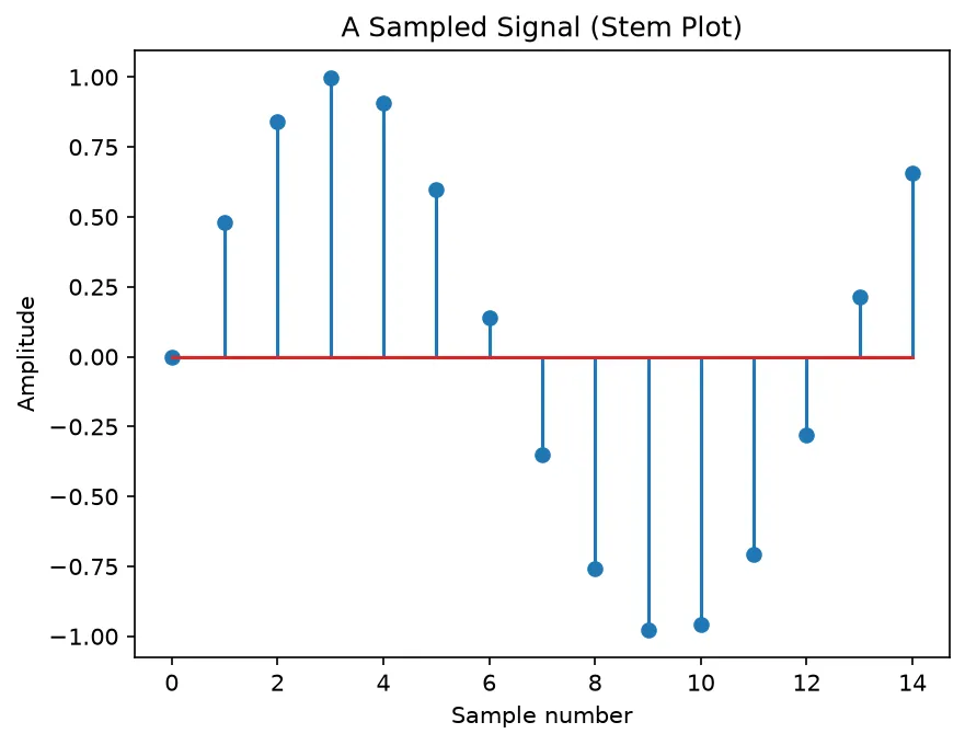
What you'll see: fifteen vertical spikes rising and falling like a sine wave, each capped with a small circle. A flat baseline runs across the middle, and spikes below it point downward where the signal goes negative.
2 Step Plots & drawstyle
A step plot draws a staircase instead of diagonal lines — the value holds flat, then jumps. This is perfect for quantities that stay constant until they change, like a price or a thermostat setting. Use ax.step(x, y, where=...): where="pre" jumps before the point, "post" jumps after, and "mid" jumps halfway between.
import matplotlib.pyplot as plt
import numpy as np

hour = np.arange(0, 9)
price = [10, 10, 12, 12, 9, 9, 9, 14, 14]

fig, ax = plt.subplots()
ax.step(hour, price, where="post", color="green",
        marker="o", label='where="post"')

# Compare with a plain line
ax.plot(hour, price, color="gray", alpha=0.4,
        linestyle="--", label="plain line")

ax.set_title("Hourly Price (Step vs Line)")
ax.set_xlabel("Hour")
ax.set_ylabel("Price ($)")
ax.legend()

plt.show()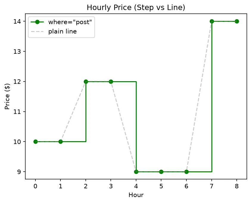
What you'll see: a green staircase that stays flat between hours and then jumps straight up or down at each change, with a marker at every point. A faint gray dashed line connects the same points diagonally so you can feel the difference between "holds then jumps" and "slides smoothly."
3 Histogram Outlines With ax.stairs()
ax.stairs() draws the outline of bars from bin edges and heights — exactly the shape a histogram makes, but as a clean line you can overlay or fill. The key rule: you pass one more edge than heights, because N bars need N+1 boundaries. Pair it with np.histogram() to outline a real distribution.
import matplotlib.pyplot as plt
import numpy as np

rng = np.random.default_rng(0)
data = rng.normal(0, 1, 1000)

counts, edges = np.histogram(data, bins=15)

fig, ax = plt.subplots()
ax.stairs(counts, edges, fill=True, alpha=0.4, color="purple",
          label="filled")
ax.stairs(counts, edges, color="purple", linewidth=2,
          label="outline")

ax.set_title("Histogram Outline With ax.stairs()")
ax.set_xlabel("Value")
ax.set_ylabel("Count")
ax.legend()

plt.show()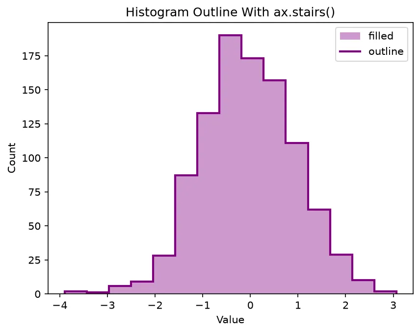
What you'll see: a bell-shaped staircase — tall in the middle, short at the edges — drawn both as a soft purple fill and as a crisp outline on top. It looks just like a histogram, but it's built from the counts and bin edges with no individual bar objects.
🎯 Your Turn: Fill in the Blanks
Replace each ___ to draw a stem plot and then a step plot of the same counts.
import matplotlib.pyplot as plt
import numpy as np

x = np.arange(1, 8)
y = [3, 5, 2, 8, 6, 4, 7]

fig, (ax1, ax2) = plt.subplots(1, 2, figsize=(10, 4))

# Left: spikes with markers
ax1.___(x, y)
ax1.set_title("Stem")

# Right: a staircase that jumps after each point
ax2.step(x, y, where=___)
ax2.set_title("Step")

plt.show()
📋 Common Errors & Quick Reference
stairs needs exactly one more edge than heights. With 10 counts you must pass 11 edges.
❌ The staircase jumps in the wrong place
Switch the where argument. Try "pre", "post", or "mid" to control when the step happens.
❌ Stem plot looks crowded
Stem plots are for a modest number of discrete samples. With hundreds of points, a line or histogram reads better.
| Call | What It Does |
|---|---|
| ax.stem(x, y) | Spike + marker per point |
| ax.step(x, y, where="post") | Staircase, jump after point |
| drawstyle="steps-pre" | Step via ax.plot() |
| ax.stairs(h, edges) | Outline from bins |
| fill=True | Solid filled stairs |
🎯 Mini-Challenge: Three Discrete Views
Show one dataset three ways — a stem plot, a step plot, and a stairs outline — in a single row so you can compare them.
import matplotlib.pyplot as plt
import numpy as np

rng = np.random.default_rng(11)
x = np.arange(0, 12)
y = rng.integers(1, 10, size=12)

fig, (ax1, ax2, ax3) = plt.subplots(1, 3, figsize=(13, 4))

# Stem
ax1.stem(x, y)
ax1.set_title("Stem")

# Step
ax2.step(x, y, where="mid", color="green", marker="o")
ax2.set_title('Step (where="mid")')

# Stairs from the same y as bar heights
edges = np.arange(0, 13)   # 13 edges for 12 heights
ax3.stairs(y, edges, fill=True, color="purple", alpha=0.4)
ax3.set_title("Stairs")

fig.suptitle("One Dataset, Three Discrete Plots")
plt.tight_layout()
plt.show()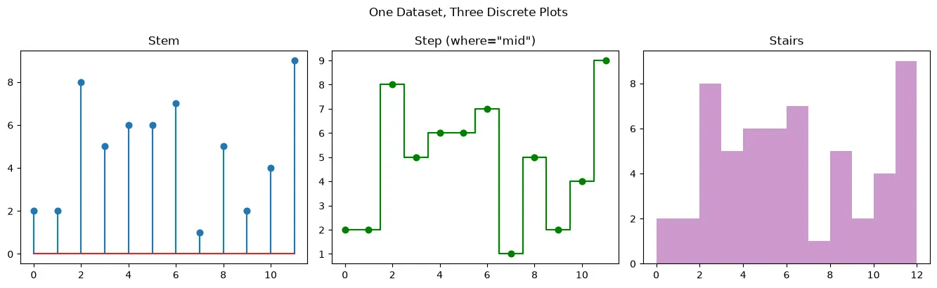
import matplotlib.pyplot as plt

x = [1, 2, 3, 4, 5]
y = [2, 5, 3, 6, 1]

fig, (left, right) = plt.subplots(1, 2, figsize=(9, 3))

container = left.stem(x, y)
right.step(x, y, where="post")

print("Stem containers:", len(left.containers))
print("Marker heights:", [int(v) for v in container.markerline.get_ydata()])
print("Baseline sits at y =", int(container.baseline.get_ydata()[0]))
print("Step line points:", len(right.lines[0].get_ydata()))
print("Step style:", right.lines[0].get_drawstyle())
print("Tallest value:", max(y), "at x =", x[y.index(max(y))])

# ✅ Expected output:
# Stem containers: 1
# Marker heights: [2, 5, 3, 6, 1]
# Baseline sits at y = 0
# Step line points: 5
# Step style: steps-post
# Tallest value: 6 at x = 4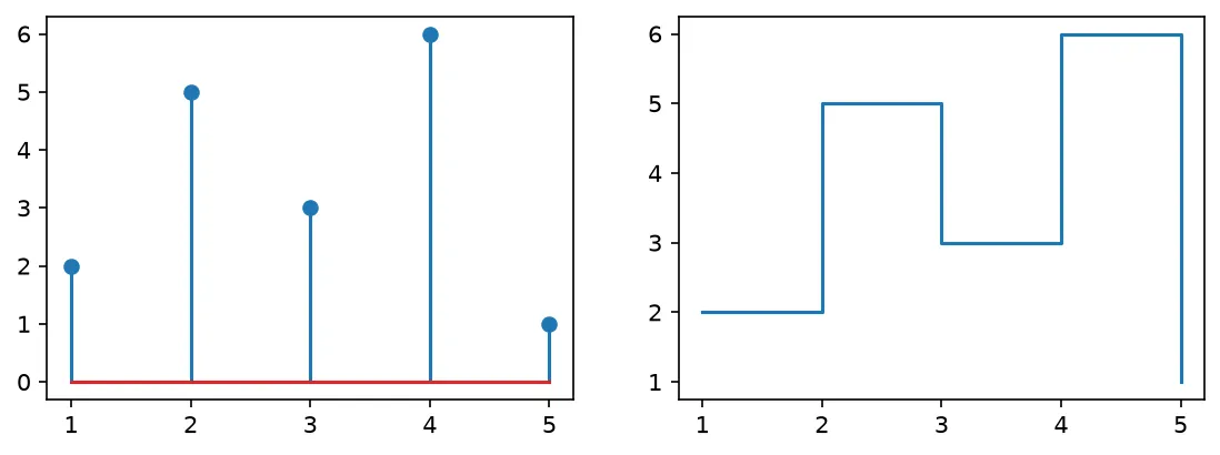
❓ Frequently Asked Questions
Lesson complete — you can plot discrete data clearly!
You drew spikes with ax.stem(), built staircases with ax.step() and drawstyle, outlined binned data with ax.stairs(), and learned when discrete plots beat a continuous line.
Practice quiz
What does a stem plot draw at each point?
- A vertical line capped with a marker
- A filled bar
- A smooth curve
- A pie slice
Answer: A vertical line capped with a marker. ax.stem draws a vertical stem from a baseline up to a marker at each value.
Which call makes a stem plot?
- ax.spike(x, y)
- ax.stem(x, y)
- ax.bar(x, y)
- ax.line(x, y)
Answer: ax.stem(x, y). ax.stem(x, y) draws a spike and marker at each (x, y).
How does ax.step() differ from ax.plot()?
- It fills the area
- It plots in 3D
- It draws a staircase instead of diagonal lines
- It uses polar axes
Answer: It draws a staircase instead of diagonal lines. ax.step() holds the value flat and then jumps, forming a staircase.
Which where= value makes the step jump after the point?
- 'pre'
- 'mid'
- 'before'
- 'post'
Answer: 'post'. where='post' holds the value then jumps after each point.
Which drawstyle on ax.plot() matches ax.step(where='post')?
- drawstyle='steps-post'
- drawstyle='post'
- drawstyle='after'
- drawstyle='jump'
Answer: drawstyle='steps-post'. ax.plot(x, y, drawstyle='steps-post') produces the same staircase.
What does ax.stairs() draw?
- A scatter of points
- The outline of bars from bin edges and heights
- A smooth spline
- A polar curve
Answer: The outline of bars from bin edges and heights. ax.stairs(counts, edges) outlines histogram-shaped bars from edges and heights.
How many edges does ax.stairs() need for N heights?
- N - 1 edges
- N edges
- N + 1 edges
- 2N edges
Answer: N + 1 edges. N bars need N+1 boundaries, so you pass one more edge than heights.
Which where= value jumps halfway between points?
- 'mid'
- 'half'
- 'center'
- 'between'
Answer: 'mid'. where='mid' makes the step jump halfway between each pair of points.
Which argument fills the area under ax.stairs()?
- solid=True
- shade=True
- area=True
- fill=True
Answer: fill=True. Pass fill=True to draw solid filled stairs.
When is a stem or step plot a poor choice?
- For a few discrete samples
- For hundreds of points where a line reads better
- For sampled signals
- For stepwise prices
Answer: For hundreds of points where a line reads better. With hundreds of points a stem plot looks crowded; a line or histogram is clearer.
Continue this course
- Previous: Filling Areas (fill_between)
- Next: Polar Plots — Plot in polar coordinates — radar-style and circular data
- Quick reference: Matplotlib cheat sheet
Frequently asked questions
What is a stem plot used for?
A stem plot draws a vertical line (a stem) from a baseline up to each data point, capped with a marker. It is the standard way to show a discrete signal — values that exist only at specific points rather than a continuous curve. Think of digital samples, counts per category, or the spikes of a signal.
What is the difference between ax.step() and ax.plot()?
ax.plot() draws straight diagonal lines connecting your points. ax.step() instead draws a staircase: the line stays flat at each value and then jumps to the next. Use a step plot when the value holds constant between samples — like a thermostat setting or a price that only changes at certain times.
What does ax.stairs() do that ax.step() does not?
ax.stairs() is designed for histogram-style outlines: you give it the bin edges and the height of each bin, and it draws the outline of those bars without filling them. ax.step() takes x and y points, while ax.stairs() takes one more edge than heights, matching how bin boundaries work.
When should I use a discrete plot instead of a continuous line?
Use a discrete plot (stem, step, or stairs) when the data only makes sense at specific points or holds steady between changes. A continuous line implies the value smoothly varies everywhere in between, which can mislead for sampled signals, counts, or stepwise quantities.