Stack Plots & Area Charts
Reviewed & published by Brayan K
A stack plot layers several filled series on top of one another so the top edge traces the running total while each colored band shows how much one series contributes over time.
Part of the free Matplotlib course at LearnCodingFast — hands-on lessons with worked examples and the output they print, plus practice exercises and a quick quiz.
In this lesson you'll fill the area under a single curve, stack multiple series with ax.stackplot(), add a legend, normalize to a 100% chart, and change the baseline.
What You'll Learn in This Lesson
- Filling a simple area under a curve
- Stacking series with ax.stackplot()
- Labeling layers and adding a legend
- Reading the total from the top edge
- Normalizing to a 100% stacked chart
- Switching the baseline for a streamgraph
1 A Simple Area Chart
Before stacking many series, start with one. An area chart is just a line plot with the space beneath it filled. You can build it with ax.fill_between(x, y) or, for a single series, with ax.stackplot(x, y). Both shade everything from the curve down to zero, giving a sense of volume rather than just a thin line.
import matplotlib.pyplot as plt
import numpy as np

days = np.arange(1, 13)
visitors = [120, 150, 170, 140, 200, 230, 260, 240, 280, 300, 330, 360]

fig, ax = plt.subplots()
ax.stackplot(days, visitors, color="mediumseagreen", alpha=0.7)
ax.plot(days, visitors, color="darkgreen")   # crisp top edge

ax.set_title("Daily Website Visitors")
ax.set_xlabel("Day")
ax.set_ylabel("Visitors")

plt.show()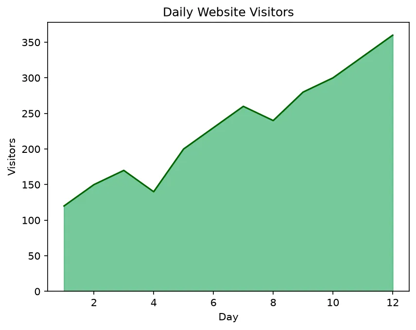
What you'll see: a green filled region climbing from left to right, capped by a darker green line that traces the visitor count. The filled body makes the upward trend feel substantial — you see growing volume, not just a rising line.
2 Stacking Multiple Series
Pass several y arrays to ax.stackplot() and Matplotlib layers them automatically: the first series sits on the bottom, the next stacks on top, and so on. The top edge of the whole stack shows the total. Add a labels list and call ax.legend() so each colored band is named.
import matplotlib.pyplot as plt
import numpy as np

years = np.arange(2018, 2025)
solar = [5, 8, 12, 18, 26, 35, 48]
wind  = [20, 24, 28, 30, 33, 36, 40]
hydro = [15, 15, 16, 16, 17, 17, 18]

fig, ax = plt.subplots()
ax.stackplot(years, solar, wind, hydro,
             labels=["Solar", "Wind", "Hydro"],
             alpha=0.8)

ax.set_title("Renewable Energy Output by Source")
ax.set_xlabel("Year")
ax.set_ylabel("Output (TWh)")
ax.legend(loc="upper left")

plt.show()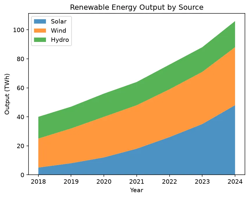
What you'll see: three colored bands stacked into one growing mountain. Hydro forms a steady base, Wind adds a thick middle layer, and Solar — the fastest-growing — fattens the top over time. The very top edge shows the combined total climbing year after year.
3 100% Stacked & the Baseline
Sometimes you care about share, not absolute size. A 100% stacked chart normalizes every column so the series always fill the full height — each band shows its percentage of the whole. Divide each series by the total at each x. You can also change the baseline argument to "sym" or "wiggle" for a centered streamgraph look.
import matplotlib.pyplot as plt
import numpy as np

months = np.arange(1, 13)
mobile  = np.array([30, 35, 40, 45, 50, 55, 60, 62, 65, 68, 70, 72])
desktop = np.array([60, 55, 52, 48, 44, 40, 36, 34, 31, 28, 26, 24])
tablet  = np.array([10, 10, 8, 7, 6, 5, 4, 4, 4, 4, 4, 4])

total = mobile + desktop + tablet
fig, ax = plt.subplots()
ax.stackplot(months,
             mobile / total * 100,
             desktop / total * 100,
             tablet / total * 100,
             labels=["Mobile", "Desktop", "Tablet"],
             alpha=0.85)

ax.set_title("Traffic Share by Device (100% Stacked)")
ax.set_xlabel("Month")
ax.set_ylabel("Share (%)")
ax.set_ylim(0, 100)
ax.legend(loc="lower left")

plt.show()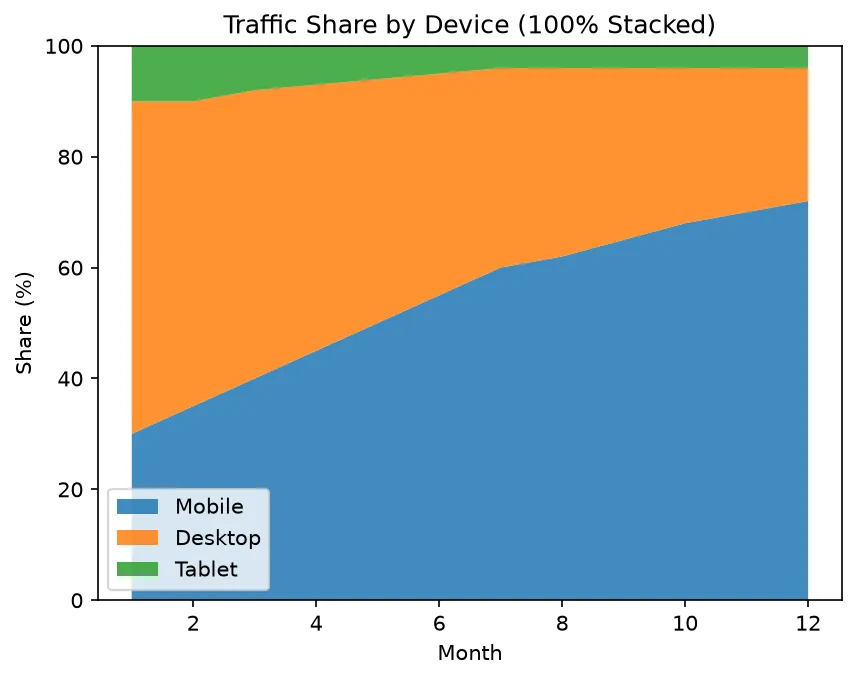
What you'll see: a chart that fills the full 0–100 height at every month. The Mobile band steadily swells while Desktop shrinks, vividly showing the shift to mobile as a change in share rather than raw counts.
🎯 Your Turn: Fill in the Blanks
Replace each ___ to stack two series and show a legend.
import matplotlib.pyplot as plt
import numpy as np

x = np.arange(1, 8)
free = [50, 55, 60, 58, 65, 70, 75]
paid = [10, 14, 18, 22, 26, 30, 36]

fig, ax = plt.subplots()

# Stack the two series with labels
ax.___(x, free, paid, labels=["Free", "Paid"], alpha=0.8)

# Show the legend so the bands are named
ax.___()

ax.set_ylabel("Users")

plt.show()
📋 Common Errors & Quick Reference
Every stacked series must be the same length as x. Double-check that all arrays line up.
❌ The legend is empty
Pass a labels list to stackplot and call ax.legend() — you need both.
❌ The 100% chart doesn't reach the top
You divided by the wrong total. Sum the series element-wise with np.array values, then divide each one by that sum.
| Call | What It Does |
|---|---|
| ax.stackplot(x, a, b) | Stack series as areas |
| labels=[...] | Name each layer |
| a / total * 100 | Normalize to percent |
| baseline="wiggle" | Streamgraph look |
| ax.fill_between(x, y) | Single filled area |
🎯 Mini-Challenge: Absolute vs Share
Show three product lines two ways: a normal stacked area chart on the left (absolute totals) and a 100% stacked chart on the right (share of the whole).
import matplotlib.pyplot as plt
import numpy as np

q = np.arange(1, 9)
basic = np.array([20, 22, 25, 28, 30, 33, 36, 40])
pro   = np.array([10, 13, 17, 22, 28, 34, 41, 50])
team  = np.array([5, 6, 8, 9, 11, 13, 16, 20])
labels = ["Basic", "Pro", "Team"]
total = basic + pro + team

fig, (ax1, ax2) = plt.subplots(1, 2, figsize=(11, 4))

# Left: absolute stacked area
ax1.stackplot(q, basic, pro, team, labels=labels, alpha=0.85)
ax1.set_title("Absolute (TWh)")
ax1.set_xlabel("Quarter")
ax1.legend(loc="upper left", fontsize=8)

# Right: 100% stacked
ax2.stackplot(q, basic/total*100, pro/total*100, team/total*100,
              labels=labels, alpha=0.85)
ax2.set_title("Share (%)")
ax2.set_xlabel("Quarter")
ax2.set_ylim(0, 100)

fig.suptitle("Subscriptions: Totals vs Share")
plt.tight_layout()
plt.show()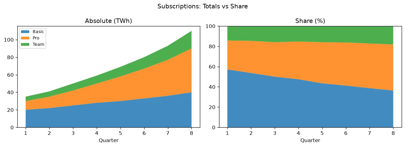
import matplotlib.pyplot as plt

years = [2021, 2022, 2023]
web = [10, 14, 18]
app = [5, 9, 15]
other = [2, 2, 3]

fig, ax = plt.subplots()
polys = ax.stackplot(years, web, app, other, labels=["web", "app", "other"])
ax.legend(loc="upper left")

totals = [w + a + o for w, a, o in zip(web, app, other)]
print("Layers:", len(polys))
print("Legend entries:", [t.get_text() for t in ax.get_legend().get_texts()])
print("Totals per year:", totals)
print("Top of the stack matches the total:", max(totals) == totals[-1])
print("Y axis reaches the total:", ax.get_ylim()[1] >= max(totals))

# ✅ Expected output:
# Layers: 3
# Legend entries: ['web', 'app', 'other']
# Totals per year: [17, 25, 36]
# Top of the stack matches the total: True
# Y axis reaches the total: True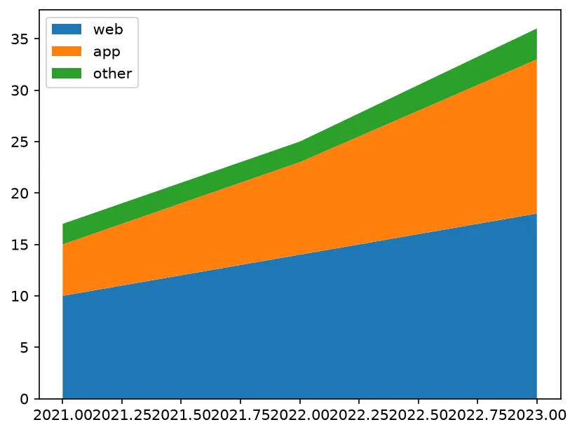
❓ Frequently Asked Questions
Lesson complete — you can show parts of a whole over time!
You filled a single area, stacked multiple series with ax.stackplot(), added a legend, normalized to a 100% chart, and learned how the baseline changes the look.
Practice quiz
Which method stacks several filled series as areas?
- ax.areaplot()
- ax.stackplot()
- ax.stack()
- ax.fillplot()
Answer: ax.stackplot(). ax.stackplot(x, a, b, c) layers the series into a stacked area chart.
What does the top edge of a stack plot show?
- The first series only
- The smallest series
- The running total
- The average
Answer: The running total. The top edge traces the running total of all stacked series.
How do you give each stacked band a name?
- Pass labels=[...] to stackplot
- Pass names=[...]
- Pass title=[...]
- Use ax.set_band()
Answer: Pass labels=[...] to stackplot. Pass a labels list to stackplot, then call ax.legend().
What two steps make a legend appear on a stack plot?
- Only call ax.legend()
- Only pass labels=
- Pass labels= and call ax.legend()
- Set baseline='legend'
Answer: Pass labels= and call ax.legend(). You need both a labels list and a call to ax.legend().
How do you make a 100% stacked chart?
- Pass percent=True
- Divide each series by the total at each x
- Use baseline='100'
- Call ax.normalize()
Answer: Divide each series by the total at each x. Normalize each series by the element-wise total so they fill the full height.
Which baseline value creates a streamgraph look?
- 'zero'
- 'edge'
- 'flat'
- 'wiggle'
Answer: 'wiggle'. baseline='wiggle' (or 'sym') centers the stack for a flowing streamgraph.
What is the default baseline for stackplot?
- 'zero'
- 'sym'
- 'wiggle'
- 'weighted_wiggle'
Answer: 'zero'. The default 'zero' stacks upward from the x-axis.
Which call fills the area under a single curve?
- ax.under(x, y)
- ax.shade(x, y)
- ax.area(x, y)
- ax.fill_between(x, y)
Answer: ax.fill_between(x, y). ax.fill_between(x, y) shades from the curve down to zero.
What error appears if a stacked series differs in length from x?
- KeyError
- ValueError: shape mismatch
- NameError
- ImportError
Answer: ValueError: shape mismatch. Every stacked series must match the length of x, or a shape mismatch ValueError occurs.
On a 100% stacked chart, what should ax.set_ylim be?
- (0, 1)
- (0, 10)
- (0, 100)
- (0, 360)
Answer: (0, 100). After normalizing to percentages, set the y-axis to (0, 100).
Continue this course
- Previous: Density: hexbin & hist2d
- Next: Checkpoint: Chart Types — Pick the right chart for the data in a multi-panel build — then a quiz
- Quick reference: Matplotlib cheat sheet
Frequently asked questions
What is a stack plot?
A stack plot draws several series stacked on top of one another as filled areas, so the top of the stack shows the running total and each colored band shows one series' contribution. Call ax.stackplot(x, series1, series2, ...) and Matplotlib layers them automatically. It is the area-chart cousin of a stacked bar chart for continuous x values like time.
How do I add a legend to a stack plot?
Pass a labels list to ax.stackplot(..., labels=['A', 'B', 'C']) and then call ax.legend(). Matplotlib matches each label to its colored band so readers can tell the layers apart. Placing the legend in an empty corner keeps it from covering the data.
How do I make a 100% stacked area chart?
Normalize each column so the series sum to one (or 100). Divide every series by the total at each x: take the element-wise sum across series, then divide each series by it and multiply by 100. After normalizing, the stack always fills the full height, showing each series' share of the whole.
What does the baseline argument do?
baseline controls where the stack is anchored. The default 'zero' stacks upward from the x-axis. 'sym' centers the stack symmetrically around zero, and 'wiggle' minimizes the slope changes to create a flowing streamgraph. Switching the baseline changes the look without changing the data.