Density: hexbin & hist2d
Reviewed & published by Brayan K
A density plot bins many data points into a grid and colors each cell by how many points it holds, revealing where data piles up even when a scatter plot would collapse into one solid blob.
Part of the free Matplotlib course at LearnCodingFast — hands-on lessons with worked examples and the output they print, plus practice exercises and a quick quiz.
In this lesson you'll build hexagonal density maps with ax.hexbin(), square ones with ax.hist2d(), add a colorbar, tune the grid size and colormap, and learn when density beats a scatter.
What You'll Learn in This Lesson
- Building a hexbin density map
- Tuning gridsize and the colormap
- Creating square-binned hist2d plots
- Adding a colorbar to read the scale
- Comparing density with a raw scatter
- Choosing density over overplotted dots
1 Your First Hexbin Map
ax.hexbin(x, y) tiles the plot with hexagons and colors each one by how many points land inside it. The gridsize argument controls how many hexagons span the width — bigger numbers mean finer detail. Pass a cmap (colormap) to choose the color scheme. Always pair it with a colorbar so the colors mean something.
import matplotlib.pyplot as plt
import numpy as np

rng = np.random.default_rng(1)
# 20,000 points clustered near the center
x = rng.normal(0, 1, 20000)
y = rng.normal(0, 1, 20000)

fig, ax = plt.subplots()
hb = ax.hexbin(x, y, gridsize=30, cmap="viridis")
fig.colorbar(hb, ax=ax, label="Point count")

ax.set_title("Hexbin Density Map")
ax.set_xlabel("x")
ax.set_ylabel("y")

plt.show()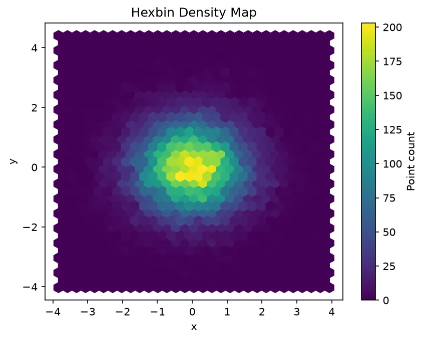
What you'll see: a roughly circular cloud of hexagons that glow brightest in the middle and fade toward the edges, showing the data piles up near the center. The colorbar on the right tells you how many points each shade represents.
2 Square Bins With ax.hist2d()
ax.hist2d(x, y) is the two-dimensional version of a histogram. It lays a rectangular grid of square bins over the data and colors each by its count. Set the number of bins with bins=. It returns several values — the counts, the two sets of edges, and the image — and you pass that last image to fig.colorbar().
import matplotlib.pyplot as plt
import numpy as np

rng = np.random.default_rng(2)
# A diagonal correlated cloud
x = rng.normal(0, 1, 30000)
y = x * 0.8 + rng.normal(0, 0.5, 30000)

fig, ax = plt.subplots()
counts, xedges, yedges, im = ax.hist2d(x, y, bins=40, cmap="plasma")
fig.colorbar(im, ax=ax, label="Point count")

ax.set_title("2D Histogram (hist2d)")
ax.set_xlabel("x")
ax.set_ylabel("y")

plt.show()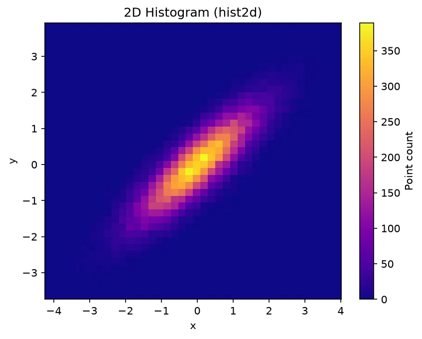
What you'll see: a bright diagonal streak running from lower-left to upper-right, made of square cells, showing that x and y rise together. The brightest cells sit along the diagonal where most points fall, and the colorbar maps each shade to a count.
3 Why Density Beats Overplotting
With a few hundred points, a scatter plot is perfect. But push it to tens of thousands and the dots merge into one solid blob — you can't tell a busy region from a packed one. This is overplotting, and density plots are the cure. Put a scatter and a hexbin side by side and the difference is obvious.
import matplotlib.pyplot as plt
import numpy as np

rng = np.random.default_rng(7)
# Two overlapping clusters
x = np.concatenate([rng.normal(-1, 0.5, 25000),
                    rng.normal(1.5, 0.7, 25000)])
y = np.concatenate([rng.normal(0, 0.5, 25000),
                    rng.normal(1, 0.7, 25000)])

fig, (ax1, ax2) = plt.subplots(1, 2, figsize=(11, 4))

# Left: overplotted scatter
ax1.scatter(x, y, s=2, alpha=0.1, color="black")
ax1.set_title("Scatter (overplotted)")

# Right: hexbin reveals two clusters
hb = ax2.hexbin(x, y, gridsize=35, cmap="inferno")
fig.colorbar(hb, ax=ax2, label="count")
ax2.set_title("Hexbin (clear)")

fig.suptitle("Density Beats Overplotting")
plt.tight_layout()
plt.show()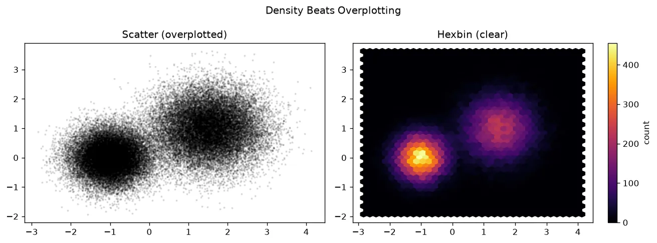
What you'll see: on the left, a near-solid gray smear where you can barely guess the shape. On the right, the hexbin clearly shows two bright hot spots — the two clusters — with a colorbar quantifying how dense each one is.
🎯 Your Turn: Fill in the Blanks
Replace each ___ to draw a hexbin map and attach a colorbar.
import matplotlib.pyplot as plt
import numpy as np

rng = np.random.default_rng(0)
x = rng.normal(0, 1, 15000)
y = rng.normal(0, 1, 15000)

fig, ax = plt.subplots()

# Make a hexbin with 25 hexagons across and the "magma" colormap
hb = ax.___(x, y, gridsize=25, cmap=___)

# Add a colorbar so the colors have meaning
fig.___(hb, ax=ax, label="count")

ax.set_title("My Hexbin Map")

plt.show()
📋 Common Errors & Quick Reference
❌ TypeError when calling fig.colorbar()
You passed the wrong object. For hist2d use the fourth return value (the image), not the counts.
❌ The map is one flat color
Your gridsize is too large or too small for the data. Try gridsize=30 and adjust until the structure appears.
❌ Low-density bins drown out the rest
Pass bins="log" to hexbin (or use a log norm) so a few crowded cells don't wash out everything else.
| Call | What It Does |
|---|---|
| ax.hexbin(x, y) | Hexagonal density map |
| gridsize=30 | Hexagons across the width |
| ax.hist2d(x, y, bins=40) | Square-binned density |
| cmap="viridis" | Pick the color scheme |
| fig.colorbar(obj, ax=ax) | Legend for the colors |
🎯 Mini-Challenge: hexbin vs hist2d
Plot the same correlated dataset two ways — hexbin on the left, hist2d on the right — each with its own colorbar, so you can judge which binning you prefer.
import matplotlib.pyplot as plt
import numpy as np

rng = np.random.default_rng(42)
x = rng.normal(0, 1, 40000)
y = 0.6 * x + rng.normal(0, 0.6, 40000)

fig, (ax1, ax2) = plt.subplots(1, 2, figsize=(11, 4))

# Left: hexagonal bins
hb = ax1.hexbin(x, y, gridsize=35, cmap="viridis")
fig.colorbar(hb, ax=ax1, label="count")
ax1.set_title("hexbin")

# Right: square bins
counts, xe, ye, im = ax2.hist2d(x, y, bins=35, cmap="viridis")
fig.colorbar(im, ax=ax2, label="count")
ax2.set_title("hist2d")

fig.suptitle("Hexagonal vs Square Bins")
plt.tight_layout()
plt.show()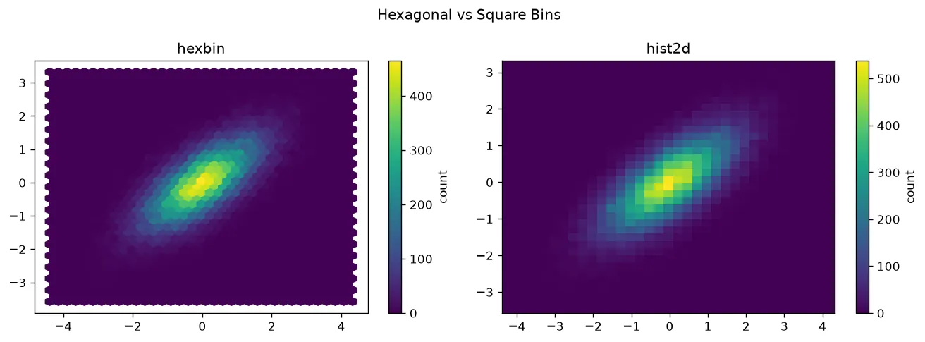
import matplotlib.pyplot as plt

xs = [1, 1, 2, 2, 2, 3, 3, 4, 5, 5, 5, 5]
ys = [1, 2, 1, 2, 2, 3, 3, 4, 5, 5, 5, 4]

fig, ax = plt.subplots()
hb = ax.hexbin(xs, ys, gridsize=3, cmap="Blues")
bar = fig.colorbar(hb, ax=ax)

counts = hb.get_array()
print("Hexagons with at least one point:", int((counts > 0).sum()))
print("Points binned:", int(counts.sum()), "of", len(xs))
print("Busiest hexagon holds:", int(counts.max()))
print("Colormap:", hb.get_cmap().name)
print("Colourbar added an axes:", len(fig.axes) == 2)

# ✅ Expected output:
# Hexagons with at least one point: 5
# Points binned: 12 of 12
# Busiest hexagon holds: 4
# Colormap: Blues
# Colourbar added an axes: True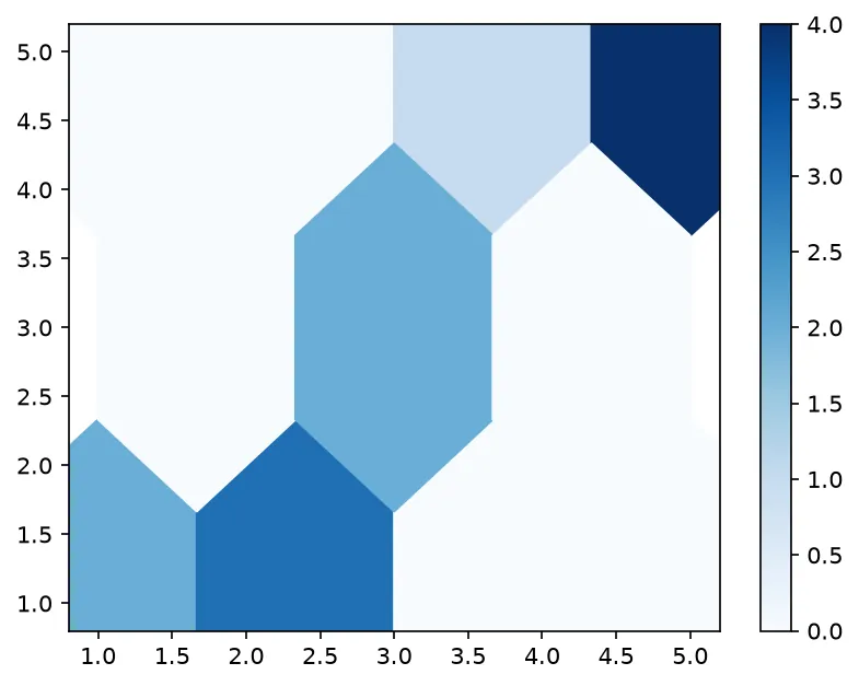
❓ Frequently Asked Questions
Lesson complete — you can map dense data!
You built hexagonal and square density maps, tuned gridsize and colormaps, added colorbars, and saw first-hand why density plots reveal structure that an overplotted scatter hides.
Practice quiz
What does ax.hexbin(x, y) draw?
- A line of best fit
- A grid of hexagons colored by point count
- A pie chart
- A 3D surface
Answer: A grid of hexagons colored by point count. hexbin tiles the area with hexagons and colors each by how many points fall inside.
Which argument controls how many hexagons span the width?
- bins
- width
- gridsize
- hexcount
Answer: gridsize. gridsize sets how many hexagons span the width; bigger means finer detail.
What is the key difference between hexbin and hist2d?
- hexbin uses hexagonal bins; hist2d uses square bins
- hexbin is 3D
- hist2d cannot show density
- They are identical
Answer: hexbin uses hexagonal bins; hist2d uses square bins. Both show 2D density, but hexbin uses hexagons while hist2d uses square bins.
Which argument sets the number of bins for ax.hist2d()?
- gridsize=
- bins=
- nbins=
- cells=
Answer: bins=. ax.hist2d(x, y, bins=40) sets the number of square bins per axis.
ax.hist2d() returns four values. Which one goes to fig.colorbar()?
- The counts
- The x edges
- The y edges
- The image (the fourth value)
Answer: The image (the fourth value). Unpack counts, xedges, yedges, im — pass the image im to fig.colorbar().
How do you add a colorbar to a hexbin plot?
- fig.colorbar(hb, ax=ax)
- ax.colorbar(hb)
- plt.legend(hb)
- hb.colorbar()
Answer: fig.colorbar(hb, ax=ax). Capture hb = ax.hexbin(...) and pass it to fig.colorbar(hb, ax=ax).
When does a density plot beat a scatter plot?
- For a few hundred points
- When so many points overlap that a scatter becomes a solid blob
- For categorical data
- For a single point
Answer: When so many points overlap that a scatter becomes a solid blob. Density plots reveal structure when overplotting turns a scatter into a blob.
What problem do hexbin and hist2d solve?
- Missing data
- Overplotting of dense scatter points
- Wrong axis labels
- Slow rendering of lines
Answer: Overplotting of dense scatter points. They cure overplotting by binning many points into colored cells.
Why do hexagonal bins often look smoother than square bins?
- They are larger
- Hexagons tile more evenly and avoid square-corner artifacts
- They use more colors
- They ignore outliers
Answer: Hexagons tile more evenly and avoid square-corner artifacts. Hexagons tile more evenly than squares, avoiding the blocky corners of square bins.
Which keeps a few crowded cells from washing out the rest in hexbin?
- gridsize=1
- bins='log' (or a log norm)
- alpha=0
- cmap='gray'
Answer: bins='log' (or a log norm). Passing bins='log' (or a log norm) compresses the scale so dense cells don't dominate.
Continue this course
- Previous: Polar Plots
- Next: Stack Plots & Area Charts — Show how parts add up over time with stacked areas
- Quick reference: Matplotlib cheat sheet
Frequently asked questions
What is a hexbin plot?
A hexbin plot divides the plotting area into a grid of hexagons and colors each one by how many data points fall inside it. It is a density map: instead of drawing thousands of overlapping dots, you see where points pile up. Call ax.hexbin(x, y) and brighter or darker hexagons mark the crowded regions.
What is the difference between hexbin and hist2d?
Both show 2D density, but hist2d uses square bins arranged in a rectangular grid, while hexbin uses hexagonal bins. Hexagons tile more evenly and avoid the visual artifacts of square corners, so hexbin often looks smoother. hist2d is the two-dimensional cousin of a regular histogram.
How do I add a colorbar to show what the colors mean?
Capture the object returned by the plotting call, then pass it to fig.colorbar(). For example hb = ax.hexbin(x, y); fig.colorbar(hb, ax=ax, label='counts'). The colorbar is a legend for color: it maps each shade to a count so readers know which regions are dense.
When should I use a density plot instead of a scatter plot?
Reach for hexbin or hist2d when you have so many points that a scatter plot turns into a solid blob — overplotting hides the structure. Density plots reveal where points concentrate even when millions overlap. For a few hundred points, a plain scatter is usually clearer.