Checkpoint: Chart Types
Reviewed & published by Brayan K
A checkpoint is a review lesson that pulls every chart type from this section together, so you can practice picking the right visualization for a given dataset and build a multi-panel figure end to end.
Part of the free Matplotlib course at LearnCodingFast — hands-on lessons with worked examples and the output they print, plus practice exercises and a quick quiz.
You'll recap box and violin plots, grouped and stacked bars, error bars, fill_between, stem and step plots, polar plots, hexbin, and stackplots — then prove it by building a small dashboard and acing a quiz.
What This Checkpoint Covers
- Recapping all eight chart types
- Matching a chart to the question it answers
- Choosing axes for a multi-panel figure
- Building a four-panel dashboard
- Reusing arange, bottom=, and bar_label
- Self-testing with a checkpoint quiz
1 Recap: Every Chart, One Job
Each chart in this section answers a specific question. The fastest way to choose is to ask what you're trying to show, then pick the chart built for it. Keep this table handy — it's the heart of the whole section.
| Chart | Key call | Use it when you want to… |
|---|---|---|
| Box / Violin | ax.boxplot / ax.violinplot | Compare distributions and spot outliers or shape |
| Grouped bars | ax.bar(x ± w/2, ...) | Compare series within each category |
| Stacked bars | ax.bar(..., bottom=) | Show a category total and its parts |
| Error bars / band | ax.errorbar / fill_between | Show uncertainty around values |
| Stem / Step | ax.stem / ax.step | Show discrete signals or stepwise values |
| Polar | projection="polar" | Plot angular, cyclic, or radar data |
| hexbin / hist2d | ax.hexbin / ax.hist2d | Map density of a huge scatter |
| Stackplot | ax.stackplot | Show parts of a whole over time |
import matplotlib.pyplot as plt
import numpy as np

rng = np.random.default_rng(0)

# Same data, two appropriate views
groups = [rng.normal(50, 8, 200),
          rng.normal(60, 5, 200),
          rng.normal(55, 12, 200)]
names = ["A", "B", "C"]

fig, (ax1, ax2) = plt.subplots(1, 2, figsize=(11, 4))
ax1.boxplot(groups, tick_labels=names)
ax1.set_title("Box: spread + outliers")

ax2.violinplot(groups, showmedians=True)
ax2.set_xticks([1, 2, 3])
ax2.set_xticklabels(names)
ax2.set_title("Violin: shape")

fig.suptitle("Pick the View That Answers Your Question")
plt.tight_layout()
plt.show()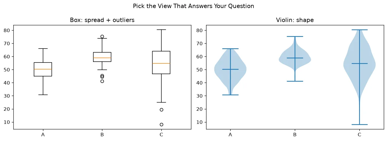
2 Build Challenge: A Four-Panel Dashboard
Time to put it together. Below is a starter that sets up a 2×2 grid of axes and hands you four datasets. Your job: pick the right chart for each panel and draw it. Think before you code — which chart answers each dataset's question? Try it yourself first, then open the solution to compare.
import matplotlib.pyplot as plt
import numpy as np

rng = np.random.default_rng(3)

# --- Four datasets, each suited to a different chart ---
# 1) Distributions of three teams  -> box or violin
teams = [rng.normal(70, 8, 150),
         rng.normal(75, 5, 150),
         rng.normal(68, 12, 150)]
team_names = ["Red", "Blue", "Green"]

# 2) Revenue split into 3 parts over 6 months -> stacked area / bars
months = np.arange(1, 7)
prod = np.array([20, 22, 25, 27, 30, 33])
serv = np.array([10, 12, 15, 18, 22, 26])
ads  = np.array([5, 6, 6, 7, 8, 10])

# 3) A huge correlated cloud -> hexbin / hist2d
hx = rng.normal(0, 1, 20000)
hy = 0.7 * hx + rng.normal(0, 0.5, 20000)

# 4) A measured trend with uncertainty -> line + band
x = np.linspace(0, 10, 50)
y = np.sqrt(x)
err = 0.15 + 0.03 * x

fig, axs = plt.subplots(2, 2, figsize=(11, 8))
ax1, ax2, ax3, ax4 = axs.flat

# TODO: draw the right chart on each axis.
# ax1: compare the three team distributions
# ax2: show the revenue split over months
# ax3: map the density of (hx, hy)
# ax4: plot y vs x with a shaded uncertainty band

fig.suptitle("Build: Choose the Right Chart for Each Panel")
plt.tight_layout()
plt.show()
The logic: distributions call for a box plot, a revenue split over time is a stackplot, a 20,000-point cloud needs hexbin, and a noisy trend wants a line with a fill_between band. Same toolbox, four different jobs.
3 Stretch It: Add a Polar Panel
One subtlety: a polar panel needs polar axes, which you request per-subplot. Use the subplot_kw trick or build a mixed figure where one axis is polar. Here's a compact example pairing a grouped bar chart with a radar-style polar bar — proof you can mix projections in one figure.
import matplotlib.pyplot as plt
import numpy as np

cats = ["Q1", "Q2", "Q3", "Q4"]
a = [120, 150, 130, 170]
b = [100, 140, 120, 160]
x = np.arange(len(cats))
width = 0.4

skills = ["Speed", "Power", "Range", "Aim", "Luck"]
vals = [8, 6, 9, 7, 5]
ang = np.linspace(0, 2 * np.pi, len(skills), endpoint=False)

fig = plt.figure(figsize=(11, 4))

# Left: a normal grouped bar chart
ax1 = fig.add_subplot(1, 2, 1)
ax1.bar(x - width/2, a, width, label="2023")
ax1.bar(x + width/2, b, width, label="2024")
ax1.set_xticks(x)
ax1.set_xticklabels(cats)
ax1.set_title("Grouped Bars")
ax1.legend(fontsize=8)

# Right: a polar bar chart in the same figure
ax2 = fig.add_subplot(1, 2, 2, projection="polar")
ax2.bar(ang, vals, width=2*np.pi/len(skills),
        color="seagreen", alpha=0.6)
ax2.set_xticks(ang)
ax2.set_xticklabels(skills)
ax2.set_title("Polar Bars")

fig.suptitle("Mixing Projections in One Figure")
plt.tight_layout()
plt.show()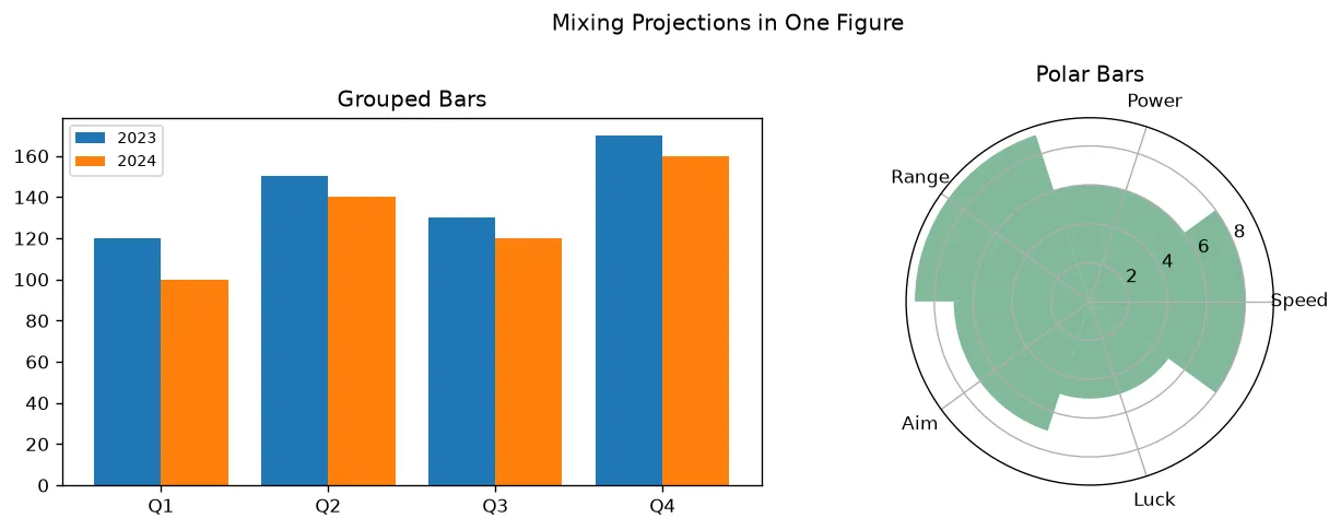
What you'll see: a normal grouped bar chart on the left and a green radar-style polar bar chart on the right, living happily in one figure — exactly the building block of a real dashboard.
🎯 Your Turn: Fill in the Blanks
Replace each ___ to pick the right call for each panel: a density map and a stacked area chart.
import matplotlib.pyplot as plt
import numpy as np

rng = np.random.default_rng(1)
px = rng.normal(0, 1, 12000)
py = rng.normal(0, 1, 12000)

t = np.arange(1, 7)
free = [40, 44, 50, 55, 60, 66]
paid = [10, 14, 18, 24, 30, 38]

fig, (ax1, ax2) = plt.subplots(1, 2, figsize=(11, 4))

# Panel 1: density of a big point cloud
ax1.___(px, py, gridsize=25, cmap="viridis")
ax1.set_title("Density")

# Panel 2: parts of a whole over time
ax2.___(t, free, paid, labels=["Free", "Paid"], alpha=0.8)
ax2.legend(fontsize=8)
ax2.set_title("Stacked Area")

plt.tight_layout()
plt.show()
📋 Common Errors & Quick Reference
❌ AttributeError on a polar method
You called set_theta_zero_location on normal axes. Create the axis with projection="polar" first.
❌ Panels overlap or labels get cut off
Call plt.tight_layout() (or fig.tight_layout()) after drawing all panels to space them out.
❌ Wrong chart for the question
If a scatter is a blob, switch to density; if you need parts of a whole, stack; if comparing distributions, use box or violin.
| Goal | Reach for |
|---|---|
| Compare distributions | boxplot / violinplot |
| Parts of a whole over time | stackplot |
| Dense scatter | hexbin / hist2d |
| Uncertainty | errorbar / fill_between |
| Cyclic / angular data | projection="polar" |
🎯 Mini-Challenge: A Three-Panel Report
Build a one-row report: error bars for measured points, a stacked bar of a budget, and a hexbin density map — each chosen for its data.
import matplotlib.pyplot as plt
import numpy as np

rng = np.random.default_rng(8)

# Panel 1: measured points with error bars
x = np.arange(1, 7)
y = np.array([2, 4, 5, 4, 6, 7])
err = np.array([0.4, 0.5, 0.3, 0.6, 0.4, 0.5])

# Panel 2: a stacked budget
cats = ["Jan", "Feb", "Mar"]
rent = np.array([1200, 1200, 1200])
food = np.array([400, 450, 380])

# Panel 3: a dense cloud
dx = rng.normal(0, 1, 15000)
dy = 0.5 * dx + rng.normal(0, 0.6, 15000)

fig, (ax1, ax2, ax3) = plt.subplots(1, 3, figsize=(14, 4))

ax1.errorbar(x, y, yerr=err, fmt="-o", capsize=4, color="purple")
ax1.set_title("Error Bars")

ax2.bar(cats, rent, label="Rent")
ax2.bar(cats, food, bottom=rent, label="Food")
ax2.set_title("Stacked Budget")
ax2.legend(fontsize=8)

hb = ax3.hexbin(dx, dy, gridsize=30, cmap="inferno")
fig.colorbar(hb, ax=ax3, label="count")
ax3.set_title("Density")

fig.suptitle("A Three-Panel Report")
plt.tight_layout()
plt.show()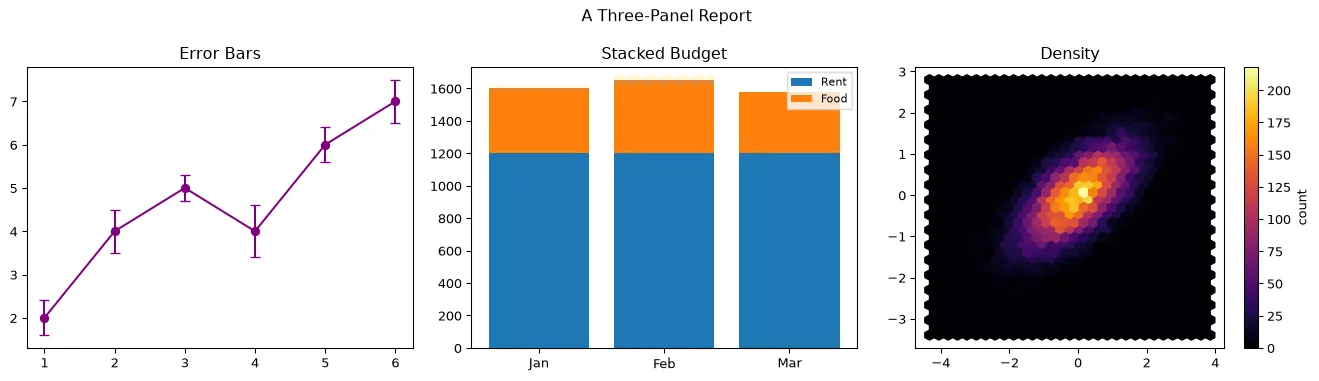
import matplotlib.pyplot as plt

data = {"line": [1, 4, 9, 16], "bar": [3, 5, 2, 6], "scatter": [(1, 2), (2, 4), (3, 1), (4, 5)]}

fig, axes = plt.subplots(1, 3, figsize=(11, 3))

axes[0].plot(data["line"])
axes[1].bar(range(4), data["bar"])
axes[2].scatter([p[0] for p in data["scatter"]], [p[1] for p in data["scatter"]])

for a, name in zip(axes, ["line", "bar", "scatter"]):
    a.set_title(name)

print("Panels:", len(fig.axes))
print("Titles:", [a.get_title() for a in axes])
print("Line points:", len(axes[0].lines[0].get_ydata()))
print("Bars:", len(axes[1].patches))
print("Scatter points:", len(axes[2].collections[0].get_offsets()))
print("Each panel got exactly one kind of plot:", [len(axes[0].lines), len(axes[1].patches), len(axes[2].collections)])

# ✅ Expected output:
# Panels: 3
# Titles: ['line', 'bar', 'scatter']
# Line points: 4
# Bars: 4
# Scatter points: 4
# Each panel got exactly one kind of plot: [1, 4, 1]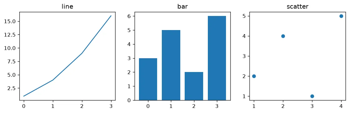
📝 Checkpoint Quiz
Answer each in your head, then click to reveal. No peeking first!
A density plot — ax.hexbin(x, y) or ax.hist2d(x, y). Both bin the points and color each cell by count so the structure shows through even when points overlap.
Grouped bars sit side by side (offset with x ± width/2) to compare series within a category. Stacked bars sit on top of each other (using bottom=) to show the category total and its breakdown.
A violin plot. It draws a smoothed density curve, so a bimodal distribution shows two bulges, while a box plot would flatten it into a single box.
Use ax.fill_between(x, y - err, y + err, alpha=0.3) to wrap the line in a translucent confidence band — cleaner than dozens of individual error bars for dense data.
projection="polar" — passed via subplot_kw={"projection": "polar"} to plt.subplots() or to fig.add_subplot(). Then you plot with angle (theta) and radius (r).
A 100% stacked area chart — normalize each series by the column total (series / total * 100) and draw with ax.stackplot() so the bands always fill the full height and reveal share.
❓ Frequently Asked Questions
Checkpoint complete — you can choose and combine chart types!
You recapped all eight chart types, matched each to the question it answers, built a multi-panel dashboard, mixed Cartesian and polar projections, and tested yourself with the quiz.
Practice quiz
You have 50,000 (x, y) points and a scatter plot looks like a solid blob. What should you switch to?
- A bigger figure
- A pie chart
- A density plot like hexbin or hist2d
- A box plot
Answer: A density plot like hexbin or hist2d. Density plots (hexbin/hist2d) bin the points and color each cell by count, so structure shows through even when points overlap.
What is the difference between grouped and stacked bars?
- Grouped sit side by side; stacked sit on top using bottom=
- They are identical
- Stacked bars sit side by side
- Grouped bars require a colorbar
Answer: Grouped sit side by side; stacked sit on top using bottom=. Grouped bars are offset side by side (x ± width/2) to compare series; stacked bars use bottom= to show a total and its parts.
Which chart reveals a bimodal distribution that a box plot would hide?
- A bar chart
- A stem plot
- A polar plot
- A violin plot
Answer: A violin plot. A violin plot draws a smoothed density curve, so two peaks appear as two bulges, while a box plot flattens them into one box.
How do you shade the uncertainty band around a smooth trend line?
- ax.errorbar on every point
- ax.fill_between(x, y - err, y + err, alpha=0.3)
- ax.hexbin(x, y)
- ax.stackplot(x, y)
Answer: ax.fill_between(x, y - err, y + err, alpha=0.3). fill_between wraps the line in a translucent band between y - err and y + err, cleaner than many individual error bars.
What single keyword turns normal axes into polar axes?
- projection="polar"
- polar=True on plot
- kind="polar"
- radial=True
Answer: projection="polar". Pass projection="polar" to add_subplot or via subplot_kw to plt.subplots, then plot with theta and r.
Which chart best shows parts of a whole changing over time?
- A scatter plot
- A box plot
- A stackplot (stacked area)
- A hexbin
Answer: A stackplot (stacked area). stackplot stacks series so you see both the total and each component's share over time.
Which call draws stacked bars by placing one series on top of another?
- ax.bar(x ± width/2, ...)
- ax.bar(..., bottom=)
- ax.barh(...)
- ax.hist(...)
Answer: ax.bar(..., bottom=). Passing bottom= (the cumulative height of prior series) stacks each bar on top of the previous one.
Which chart pair is right for comparing the distribution of several groups?
- pie and donut
- stem and step
- hexbin and hist2d
- boxplot and violinplot
Answer: boxplot and violinplot. boxplot and violinplot both summarize distributions; box shows quartiles/outliers, violin shows full shape.
What does ax.step() emphasize compared to ax.plot()?
- Smooth curves
- Stepwise, discrete-level changes
- Density of points
- Angular data
Answer: Stepwise, discrete-level changes. step draws horizontal-then-vertical segments, ideal for discrete or stepwise signals that hold a value then jump.
For a dense scatter of 20,000 points, which gives a readable density map?
- ax.scatter with small markers
- ax.plot with a line
- ax.hexbin with gridsize
- ax.bar
Answer: ax.hexbin with gridsize. hexbin aggregates points into hexagonal bins colored by count, revealing density that an overplotted scatter hides.
Continue this course
- Previous: Stack Plots & Area Charts
- Next: Complex Layouts with GridSpec — Build magazine-style layouts with GridSpec and subplot_mosaic
- Quick reference: Matplotlib cheat sheet
Frequently asked questions
How do I choose the right chart type for my data?
Match the chart to the question. Use a box or violin plot to compare distributions, grouped or stacked bars to compare categories, error bars or a fill_between band to show uncertainty, a stem or step plot for discrete signals, a polar plot for angular or cyclic data, hexbin or hist2d for dense scatter, and a stackplot to show parts of a whole over time.
When should I use density plots instead of a scatter plot?
Switch to hexbin or hist2d once a scatter plot becomes an overplotted blob — usually beyond a few thousand points. Density plots bin the points and color each cell by count, so concentrated regions stay visible even when millions of points overlap.
What is the difference between grouped and stacked bars again?
Grouped bars sit side by side so you compare individual series within each category, answering 'which is biggest here?'. Stacked bars sit on top of each other so you see the category total and its breakdown, answering 'what's the total and how does it split?'.
Can I combine several chart types in one figure?
Yes. Create multiple axes with plt.subplots(rows, cols) and draw a different chart on each one. This is exactly how you build a dashboard — a box plot in one panel, a stacked area in another, a hexbin in a third — each chosen to fit the data it shows.