Displaying Images & Matrices (imshow)
Reviewed & published by Brayan K
imshow renders a 2D array as a grid of colored pixels, turning a matrix, heatmap, or image into a picture where each cell's value becomes a color.
Part of the free Matplotlib course at LearnCodingFast — hands-on lessons with worked examples and the output they print, plus practice exercises and a quick quiz.
In this lesson you'll display arrays with ax.imshow(), control origin, extent, aspect, and interpolation, compare it with pcolormesh, and add a colorbar.
What You'll Learn in This Lesson
- Drawing a 2D array with ax.imshow()
- Choosing a colormap and adding a colorbar
- Flipping the y-axis with origin
- Mapping pixels to data units with extent
- Controlling shape with aspect and interpolation
- When pcolormesh is the better choice
1 An Array as an Image
Hand ax.imshow() any 2D array and it paints one colored pixel per cell, mapping values to colors through the colormap. It returns a mappable, so you can attach a colorbar just like with the heatmaps you saw earlier. This is the simplest way to see the contents of a matrix.
import matplotlib.pyplot as plt
import numpy as np

# A small 2D array of numbers
matrix = np.array([
    [1, 2, 3, 4],
    [5, 6, 7, 8],
    [9, 10, 11, 12],
])

fig, ax = plt.subplots(figsize=(5, 4), constrained_layout=True)
im = ax.imshow(matrix, cmap="viridis")   # each cell becomes a colored pixel
fig.colorbar(im, ax=ax, label="Value")

ax.set_title("A 3x4 Matrix as an Image")
plt.show()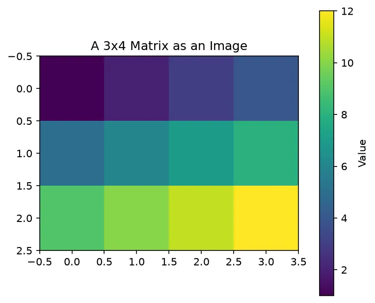
What you'll see: a 3-row, 4-column grid of squares shaded from dark purple (1) to bright yellow (12), with a colorbar translating each shade back into its number.
2 Origin: Which Way Is Up?
By default imshow uses origin="upper", putting row 0 at the top — the image convention. Switch to origin="lower" to put row 0 at the bottom, matching the usual math orientation where y grows upward. Getting this right keeps your data from appearing upside-down.
import matplotlib.pyplot as plt
import numpy as np

data = np.arange(16).reshape(4, 4)

fig, (ax1, ax2) = plt.subplots(1, 2, figsize=(9, 4), constrained_layout=True)

# Default origin is "upper": row 0 sits at the TOP
ax1.imshow(data, cmap="plasma", origin="upper")
ax1.set_title('origin="upper" (default)')

# origin="lower" flips it so row 0 sits at the BOTTOM
ax2.imshow(data, cmap="plasma", origin="lower")
ax2.set_title('origin="lower"')

plt.show()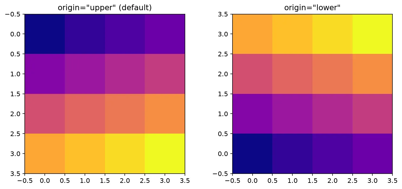
What you'll see: the same 4×4 gradient twice. On the left the brightest cell (15) sits in the bottom-right with the count rising downward; on the right the array is flipped vertically so the count rises upward.
3 extent, aspect & interpolation
Three more arguments give you full control. extent=[xmin, xmax, ymin, ymax] maps the array onto real data coordinates so the axes show units, not pixel indices. aspect="auto" lets the image stretch to fill the Axes (use "equal" for square pixels). interpolation smooths the pixels — "nearest" keeps them blocky, "bilinear" blends them.
import matplotlib.pyplot as plt
import numpy as np

x = np.linspace(-2, 2, 100)
y = np.linspace(-2, 2, 100)
X, Y = np.meshgrid(x, y)
Z = np.sin(X**2 + Y**2)

fig, ax = plt.subplots(figsize=(6, 5), constrained_layout=True)

# extent maps the array onto real x/y data coordinates;
# aspect="auto" lets the image stretch to fill the Axes
im = ax.imshow(Z, cmap="coolwarm", origin="lower",
               extent=[-2, 2, -2, 2], aspect="auto",
               interpolation="bilinear")
fig.colorbar(im, ax=ax, label="Z")

ax.set_xlabel("x")
ax.set_ylabel("y")
ax.set_title("imshow with extent and interpolation")
plt.show()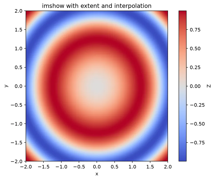
What you'll see: a smooth, rippling red-and-blue pattern of concentric waves, with the x and y axes labeled from -2 to 2 (thanks to extent) and the pixels blended into a continuous surface by bilinear interpolation.
🎯 Your Turn: Fill in the Blanks
Replace each ___ to display a random grid with the magma colormap and a colorbar.
import matplotlib.pyplot as plt
import numpy as np

grid = np.random.default_rng(0).random((6, 6))

fig, ax = plt.subplots(figsize=(5, 4), constrained_layout=True)

# Show the grid as an image using the "magma" colormap
im = ax.___(grid, cmap="magma")

# Attach a colorbar to that image
fig.___(im, ax=ax)

ax.set_title("Random Grid")
plt.show()
Hint: the image method is imshow, and the figure method that adds the legend strip is colorbar.
📋 Common Errors & Quick Reference
❌ My image looks upside-down
You expected math orientation but got the image default. Add origin="lower" so row 0 sits at the bottom.
❌ TypeError: Invalid shape for image data
imshow needs a 2D array (or a 3D RGB array). A 1D list won't work — reshape it first with .reshape(rows, cols).
❌ The image is squished or stretched
Set aspect: use "equal" to keep pixels square, or "auto" to let the image fill the Axes.
| Argument | What It Controls |
|---|---|
| cmap= | Which colormap maps value to color |
| origin= | Whether row 0 is top or bottom |
| extent= | Data coordinates of the edges |
| interpolation= | Blocky vs smoothed pixels |
🏆 Mini Challenge: Annotated Heatmap
Build a 5×5 heatmap with day labels on both axes and the numeric value written inside every cell.
import matplotlib.pyplot as plt
import numpy as np

labels = ["Mon", "Tue", "Wed", "Thu", "Fri"]
data = np.random.default_rng(1).integers(0, 100, (5, 5))

fig, ax = plt.subplots(figsize=(6, 5), constrained_layout=True)
im = ax.imshow(data, cmap="YlGnBu")
fig.colorbar(im, ax=ax, label="Score")

ax.set_xticks(range(5), labels)
ax.set_yticks(range(5), labels)

# Write each value into its cell
for i in range(5):
    for j in range(5):
        ax.text(j, i, str(data[i, j]), ha="center", va="center",
                color="black", fontsize=8)

ax.set_title("Weekly Score Heatmap")
plt.show()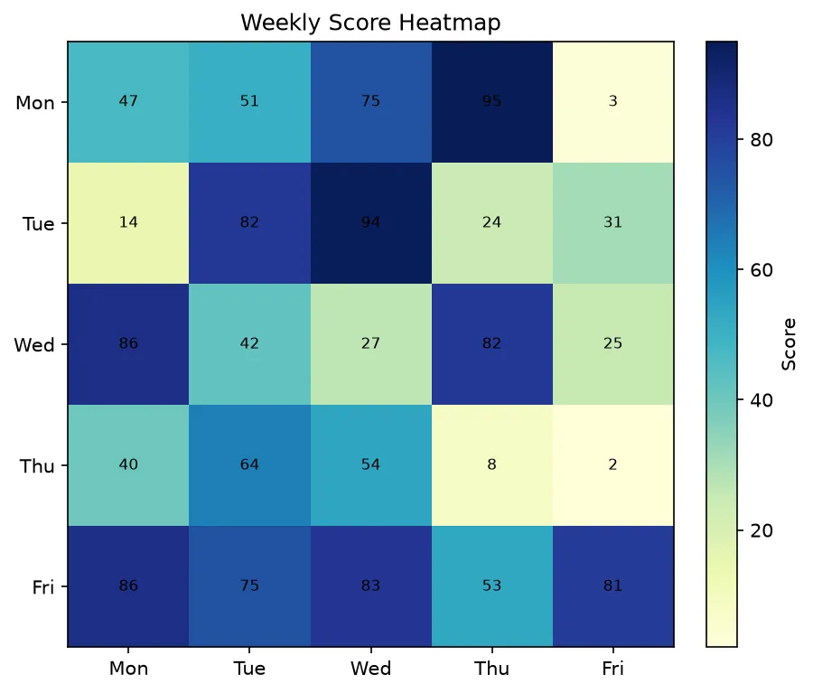
import matplotlib.pyplot as plt

grid = [[0, 1, 2],
        [3, 4, 5],
        [6, 7, 8]]

fig, ax = plt.subplots()
im = ax.imshow(grid, cmap="viridis", vmin=0, vmax=8, origin="upper")

print("Shape:", im.get_array().shape)
print("Colour limits:", [int(v) for v in im.get_clim()])
print("Origin:", im.origin)
print("Top-left cell is grid[0][0]:", grid[0][0])
print("Extent (left, right, bottom, top):", [round(v, 1) for v in im.get_extent()])
print("Aspect:", ax.get_aspect())

# ✅ Expected output:
# Shape: (3, 3)
# Colour limits: [0, 8]
# Origin: upper
# Top-left cell is grid[0][0]: 0
# Extent (left, right, bottom, top): [-0.5, 2.5, 2.5, -0.5]
# Aspect: 1.0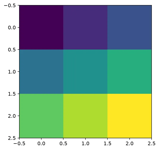
❓ Frequently Asked Questions
Lesson complete — you can turn any matrix into a picture!
You displayed arrays with ax.imshow(), flipped the y-axis with origin, mapped pixels to data units with extent, and tuned shape with aspect and interpolation.
Practice quiz
What does ax.imshow() draw?
- A line plot
- A 2D array as a grid of colored pixels
- A 3D mesh
- A pie chart
Answer: A 2D array as a grid of colored pixels. imshow renders a 2D array as colored pixels, one rectangle per cell.
What is the default value of the origin argument?
- 'lower'
- 'center'
- 'upper'
- 'auto'
Answer: 'upper'. The default origin='upper' places row 0 at the top, the image convention.
What does origin='lower' do?
- Puts row 0 at the bottom (math orientation)
- Puts row 0 at the top
- Flips left-right
- Reverses the colormap
Answer: Puts row 0 at the bottom (math orientation). origin='lower' places row 0 at the bottom, matching y-increases-upward math orientation.
What does extent=[xmin, xmax, ymin, ymax] do?
- Sets the colormap range
- Maps the array onto real data coordinates
- Sets the DPI
- Chooses interpolation
Answer: Maps the array onto real data coordinates. extent maps the array onto data coordinates so axes show units, not pixel indices.
Which aspect value lets the image stretch to fill the Axes?
- 'equal'
- 'auto'
- 'square'
- 'fit'
Answer: 'auto'. aspect='auto' lets the image stretch; 'equal' keeps pixels square.
Which interpolation keeps the pixels blocky (no smoothing)?
- 'bilinear'
- 'bicubic'
- 'nearest'
- 'gaussian'
Answer: 'nearest'. interpolation='nearest' keeps pixels blocky; 'bilinear' blends them.
When should you use pcolormesh instead of imshow?
- For a plain square-celled matrix
- For irregular or non-uniform grids with explicit edge coordinates
- For 1D data
- For faster rendering of images
Answer: For irregular or non-uniform grids with explicit edge coordinates. pcolormesh accepts explicit X/Y edges, handling irregular grids imshow cannot.
imshow returns a mappable. How do you add a colorbar to it?
- fig.colorbar(im, ax=ax)
- ax.legend(im)
- im.colorbar()
- plt.key(im)
Answer: fig.colorbar(im, ax=ax). Capture im = ax.imshow(...) and pass it to fig.colorbar(im, ax=ax).
A color photo passed to imshow is what shape?
- (height, width)
- (height, width, 3) for RGB channels
- (3, height)
- (width,)
Answer: (height, width, 3) for RGB channels. An RGB photo is a 3D array (height, width, 3); imshow displays it with no colormap.
If your image looks upside-down (you expected math orientation), you should...
- Set aspect='equal'
- Add origin='lower'
- Change the cmap
- Call colorbar()
Answer: Add origin='lower'. Add origin='lower' so row 0 sits at the bottom in math orientation.
Continue this course
- Previous: Contour & Filled Contour Plots
- Next: Tick Locators & Formatters — Control tick placement and format axes as %, currency, or dates
- Quick reference: Matplotlib cheat sheet
Frequently asked questions
What does ax.imshow() actually do?
imshow draws a 2D array as a grid of colored pixels: each array cell becomes one rectangle, and its value is mapped to a color through the chosen colormap. It is the go-to tool for heatmaps, matrices, and real images stored as arrays.
What is the difference between origin='upper' and origin='lower'?
By default imshow uses origin='upper', placing row 0 of the array at the top of the figure — the convention for images, where the first row is the top scanline. origin='lower' flips it so row 0 sits at the bottom, which matches the usual math orientation where y increases upward.
When should I use pcolormesh instead of imshow?
imshow assumes evenly spaced, square-ish cells and is fast and simple for regular grids and images. pcolormesh accepts explicit X and Y edge coordinates, so it handles irregular or non-uniform grids that imshow cannot. For a plain matrix or photo, imshow is simpler; for a warped or unevenly spaced grid, reach for pcolormesh.
How do extent and aspect control the image?
extent=[xmin, xmax, ymin, ymax] maps the array onto real data coordinates so the axes show meaningful units instead of pixel indices. aspect='auto' lets the image stretch to fill the Axes, while aspect='equal' keeps pixels square. Together they control how the array is positioned and proportioned.