Histograms
Reviewed & published by Brayan K
Matplotlib is a Python library for creating charts and visualizations — and the histogram is the tool you reach for when you want to see the shape of a single numeric variable.
Part of the free Matplotlib course at LearnCodingFast — hands-on lessons with worked examples and the output they print, plus practice exercises and a quick quiz.
In this lesson you'll bucket data into bins, tune the bin count, normalize with density, and overlay two distributions to compare them.
What You'll Learn in This Lesson
- Building a histogram with plt.hist()
- Controlling detail with the bins argument
- Outlining bars with edgecolor
- Normalizing with density=True
- Overlaying two distributions with alpha
- Reading the shape of a distribution
1 Your First Histogram
A histogram takes one list of numbers, slices the range into equal bins, and counts how many values fall in each bin. Pass your data to plt.hist() and add edgecolor so the bars stay distinct.
import matplotlib.pyplot as plt
import numpy as np

# 500 exam scores centered around 70
np.random.seed(0)
scores = np.random.normal(loc=70, scale=10, size=500)

# Slice the range into 20 bins
plt.hist(scores, bins=20, edgecolor="black", color="cornflowerblue")

plt.title("Distribution of Exam Scores")
plt.xlabel("Score")
plt.ylabel("Number of Students")

plt.show()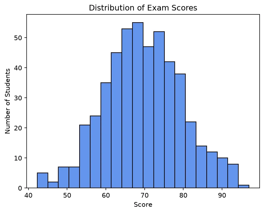
What you'll see: a bell-shaped cluster of blue bars, tallest near a score of 70 and tapering off toward 40 and 100. Each bar is outlined in black, and the y-axis tells you how many students landed in each score range.
2 Bin Count & Density
The bins argument controls resolution: fewer bins give a smooth summary, more bins reveal fine detail. Setting density=True rescales the y-axis so the bars represent probability density (total area equals 1) instead of raw counts.
import matplotlib.pyplot as plt
import numpy as np

np.random.seed(1)
data = np.random.normal(loc=0, scale=1, size=1000)

# More bins + density normalization
plt.hist(data, bins=40, density=True,
         edgecolor="black", color="mediumseagreen")

plt.title("Standard Normal Distribution (Density)")
plt.xlabel("Value")
plt.ylabel("Probability Density")

plt.show()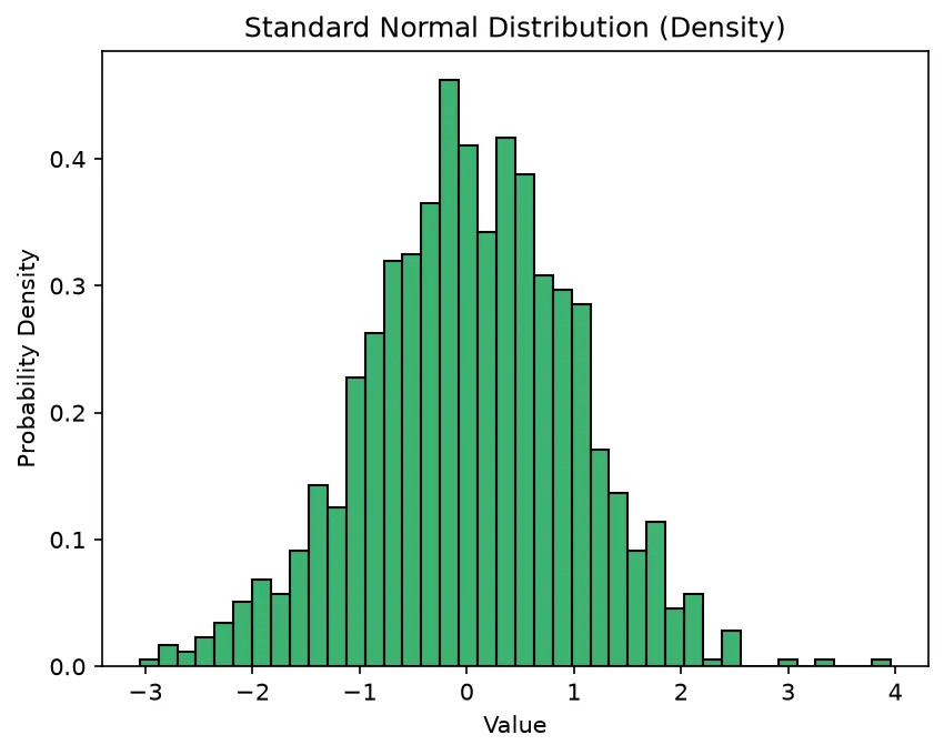
What you'll see: a finer, smoother bell curve with 40 narrow green bars peaking near 0. Because density=True is on, the y-axis now reads as probability density rather than counts, so the values are small decimals.
3 Comparing Two Distributions
To compare two groups, draw two histograms on the same axes and set alpha below 1 so the overlap is visible through the transparency. A legend tells the two groups apart.
import matplotlib.pyplot as plt
import numpy as np

np.random.seed(2)
class_a = np.random.normal(65, 8, 400)
class_b = np.random.normal(75, 8, 400)

# Same bin edges for a fair comparison
bins = np.linspace(40, 100, 25)

plt.hist(class_a, bins=bins, alpha=0.6, label="Class A", edgecolor="black")
plt.hist(class_b, bins=bins, alpha=0.6, label="Class B", edgecolor="black")

plt.title("Class A vs Class B Scores")
plt.xlabel("Score")
plt.ylabel("Count")
plt.legend()

plt.show()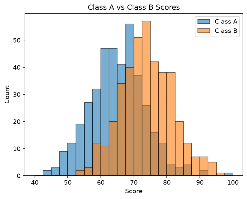
What you'll see: two semi-transparent bell shapes. Class A peaks around 65 and Class B around 75, and where they overlap in the middle the colors blend, making it obvious that Class B generally scored higher.
🎯 Your Turn: Fill in the Blanks
Replace each ___ to bucket the data into 15 outlined bins.
import matplotlib.pyplot as plt
import numpy as np

heights = np.random.normal(170, 7, 300)

# Draw a histogram with 15 bins and black edges
plt.___(heights, bins=___, edgecolor="black")

# Label the x-axis
plt.xlabel("Height (cm)")

# Display the chart
plt.___()
📋 Common Errors & Quick Reference
❌ Only one giant bar appears
You passed already-counted data. A histogram needs the raw values; it counts them for you.
❌ Bars all blur together
Add edgecolor="black" so each bin gets an outline, and lower alpha when overlaying.
| Argument | What It Does |
|---|---|
| bins=20 | Number of buckets |
| density=True | Normalize to area = 1 |
| edgecolor="black" | Outline each bar |
| alpha=0.6 | Transparency for overlap |
🏆 Mini Challenge: Commute Times
Plot the distribution of 600 commute times across 25 bins with a title and labels.
import matplotlib.pyplot as plt
import numpy as np

np.random.seed(7)
commute = np.random.normal(30, 8, 600)

plt.hist(commute, bins=25, edgecolor="black", color="indianred")

plt.title("Daily Commute Times")
plt.xlabel("Minutes")
plt.ylabel("Number of People")

plt.show()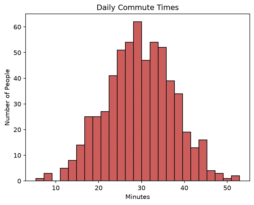
import matplotlib.pyplot as plt

ages = [12, 15, 15, 18, 21, 22, 22, 22, 25, 31, 34, 39]

fig, ax = plt.subplots()
counts, edges, patches = ax.hist(ages, bins=4, color="seagreen", edgecolor="white")

print("Bins:", len(counts))
print("Counts per bin:", [int(c) for c in counts])
print("Every value counted:", int(sum(counts)) == len(ages))
print("First bin starts at:", edges[0])
print("Last bin ends at:", edges[-1])
print("Bin width:", round(edges[1] - edges[0], 2))

# ✅ Expected output:
# Bins: 4
# Counts per bin: [4, 5, 1, 2]
# Every value counted: True
# First bin starts at: 12.0
# Last bin ends at: 39.0
# Bin width: 6.75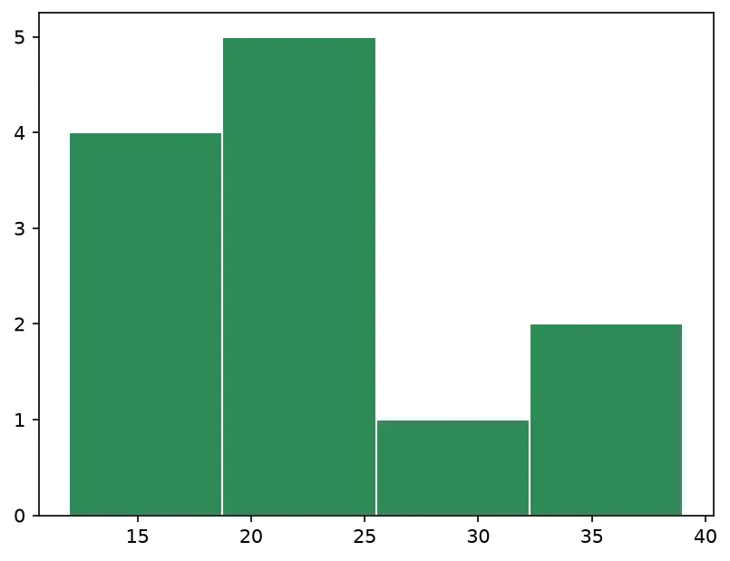
❓ Frequently Asked Questions
Lesson complete — you can read a distribution's shape!
You built histograms, tuned the bin count, normalized with density, and overlaid two groups to compare them side by side.
Practice quiz
What does a histogram show?
- The relationship between two variables
- The distribution of a single numeric variable
- A proportion as slices
- Change over exact time
Answer: The distribution of a single numeric variable. A histogram groups one numeric variable into bins to show its distribution.
Which function draws a histogram in pyplot?
- plt.bar()
- plt.hist()
- plt.histogram()
- plt.dist()
Answer: plt.hist(). plt.hist(data) slices the range into bins and counts values in each.
What does the bins argument control?
- The bar color
- The number of buckets the range is sliced into
- The figure size
- The transparency
Answer: The number of buckets the range is sliced into. bins sets how many equal-width buckets the data range is divided into.
Why pass raw values rather than pre-counted categories to plt.hist()?
- It is faster
- A histogram counts the values for you
- Counts are required
- Raw values are ignored
Answer: A histogram counts the values for you. A histogram does the counting itself; pre-counted data yields one giant bar.
What does density=True do?
- Adds more bins
- Doubles the counts
- Normalizes bars so the total area equals 1
- Removes the edges
Answer: Normalizes bars so the total area equals 1. density=True rescales the y-axis to a probability density with total area 1.
Why add edgecolor='black' to a histogram?
- To fill the bars
- To set the title
- To normalize the data
- To outline each bar so bins stay distinct
Answer: To outline each bar so bins stay distinct. Without an edge color the bars blend together; edgecolor outlines each bin.
When overlaying two histograms, which argument reveals the overlap?
- alpha below 1 (transparency)
- bins=1
- density=False
- color='black'
Answer: alpha below 1 (transparency). Setting alpha below 1 makes the overlapping region visible through transparency.
For a fair comparison of two groups, you should...
- Use different bin edges
- Use no bins
- Use the same bin edges for both
- Plot them on separate figures
Answer: Use the same bin edges for both. Shared bin edges (e.g. np.linspace) make the two distributions directly comparable.
If only one giant bar appears, the likely cause is...
- Too many bins
- You passed already-counted data instead of raw values
- edgecolor was set
- density=True
Answer: You passed already-counted data instead of raw values. Pre-counted data collapses into one bar; a histogram needs the raw values.
What is a reasonable starting number of bins to try?
- 1 to 2
- 500
- exactly 1000
- 20 to 30
Answer: 20 to 30. Around 20-30 bins is a common starting point; too few hide detail, too many add noise.
Continue this course
- Previous: Bar Charts
- Next: Scatter Plots — Plot relationships between two variables point by point
- Quick reference: Matplotlib cheat sheet › Plot Types
Frequently asked questions
What is the difference between a bar chart and a histogram?
A bar chart compares separate categories and leaves gaps between bars. A histogram shows the distribution of a single numeric variable by grouping values into ranges called bins, so the bars usually touch each other.
How do I choose the number of bins?
Pass bins= to plt.hist(). Too few bins hide detail; too many make the chart noisy. A common starting point is 20–30 bins, then adjust. You can also pass a list of explicit bin edges for full control.
What does density=True do?
By default a histogram shows raw counts on the y-axis. With density=True the bars are normalized so the total area equals 1, turning the histogram into a probability density — handy for comparing distributions of different sample sizes.
Why add edgecolor='black'?
Without an edge color the bars blend together and you cannot tell where one bin ends and the next begins. Setting edgecolor='black' outlines each bar so the buckets stay visually distinct.