Checkpoint: Data Visualization
Reviewed & published by Brayan K
A checkpoint is a chance to consolidate, where you review the data-visualization skills from the recent lessons and prove them by building one complete, polished, annotated figure of your own.
Part of the free Matplotlib course at LearnCodingFast — hands-on lessons with worked examples and the output they print, plus practice exercises and a quick quiz.
You'll recap vector fields, spines, advanced legends, inset and broken axes, patches, events, multiple figures, tables, log scales, the extra plot types, and donuts — then put them to work in a multi-step build challenge and a short quiz.
What This Checkpoint Covers
- Recapping the advanced visualization toolkit
- Choosing the right plot type for the job
- Cleaning a figure with spine tweaks
- Placing legends and annotations well
- Combining several techniques in one figure
- Self-testing with a checkpoint quiz
1 Recap: Your Visualization Toolkit
You have added a deep set of tools since the last checkpoint. Here is the quick map of what each one is for, so you can pick the right technique when you build the challenge below.
| Technique | Reach for it when… |
|---|---|
| quiver / streamplot | You have a vector field — forces, wind, flow |
| ax.spines[...] | You want a clean, minimalist frame |
| bbox_to_anchor, add_artist | The legend must sit outside or split in two |
| inset_axes / broken axis | You need a zoom-in or to span a big gap |
| patches | You want to shade or annotate a region |
| mpl_connect | The figure must react to clicks or keys |
| plt.figure / plt.close | You juggle several figure windows |
| ax.table | A chart needs its exact numbers beside it |
| set_yscale('log'/'symlog') | Data spans many orders of magnitude |
| eventplot / broken_barh / stairs | Timelines, Gantt charts, step outlines |
| pie with wedgeprops | Showing parts of a whole as a donut |
2 Warm-Up: Combine Two Techniques
Before the big build, warm up by combining a clean spine treatment with a shaded region and an annotation — three small skills working together on one line chart.
import matplotlib.pyplot as plt
import numpy as np
from matplotlib.patches import Rectangle

x = np.linspace(0, 12, 300)
y = np.sin(x) + 0.1 * x

fig, ax = plt.subplots()
ax.plot(x, y, color="navy", linewidth=2)

# Clean frame
ax.spines["top"].set_visible(False)
ax.spines["right"].set_visible(False)

# Shade a region of interest
ax.add_patch(Rectangle((4, ax.get_ylim()[0]), 3,
             ax.get_ylim()[1] - ax.get_ylim()[0],
             facecolor="gold", alpha=0.2))

# Annotate the peak inside the shaded band
peak_x = x[np.argmax(np.where((x >= 4) & (x <= 7), y, -np.inf))]
peak_y = np.sin(peak_x) + 0.1 * peak_x
ax.annotate("local peak", xy=(peak_x, peak_y),
            xytext=(peak_x + 1.5, peak_y + 1),
            arrowprops=dict(arrowstyle="->"))

ax.set_title("Spines + Highlight + Annotation")
plt.show()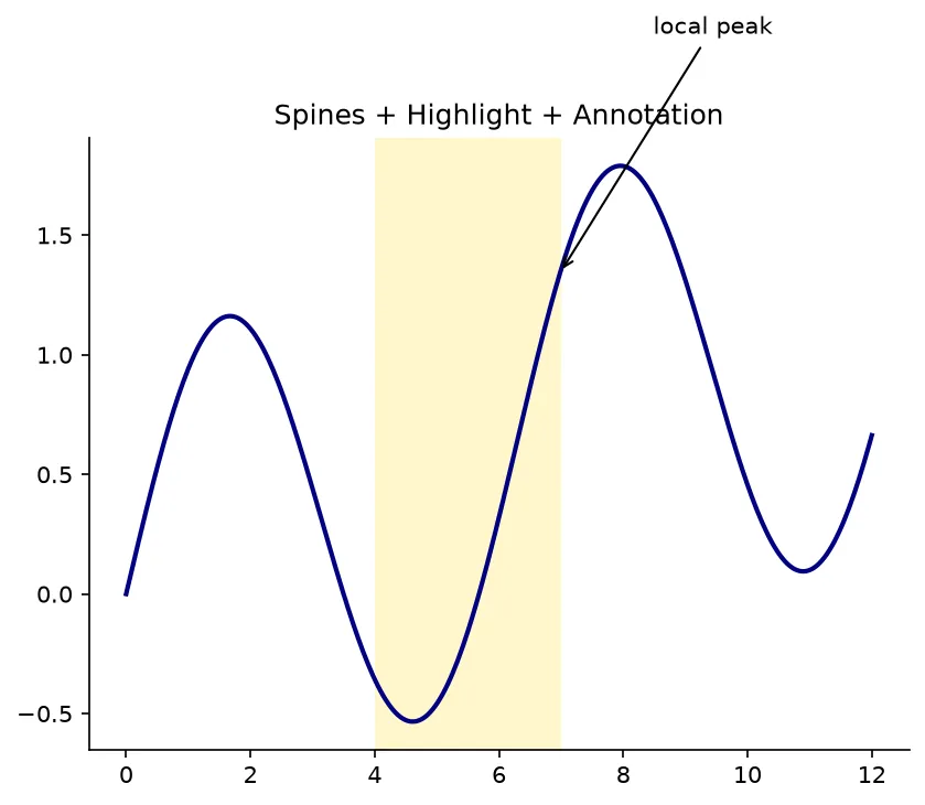
What you'll see: a navy curve on an open L-shaped frame, a gold band marking the region of interest, and an arrow labeling the local peak inside it — three techniques in one tidy figure.
3 🏗️ Build Challenge: A Polished Dashboard Figure
Build a two-panel figure for a fictional product launch. Left panel: a semilog line of daily downloads (which grow exponentially) with the top and right spines hidden and the launch day annotated. Right panel: a donut of traffic sources with percentage labels and a legend. Give the whole figure a title.
Start from the scaffold below and fill in each # TODO. Build one piece at a time and run after each. When you are done, expand the solution to compare.
import matplotlib.pyplot as plt
import numpy as np

# --- Data -----------------------------------------------------------
days = np.arange(1, 21)
downloads = 50 * 1.4 ** days          # exponential growth
sources = [52, 28, 12, 8]
source_labels = ["Search", "Social", "Direct", "Referral"]

fig, (ax_line, ax_pie) = plt.subplots(1, 2, figsize=(11, 4.5))

# --- LEFT: semilog growth line --------------------------------------
ax_line.plot(days, downloads, marker="o", color="teal")
# TODO 1: make the y-axis logarithmic

# TODO 2: hide the top and right spines of ax_line

# TODO 3: annotate day 1 as "Launch" with an arrow

ax_line.set_title("Daily Downloads (log)")
ax_line.set_xlabel("Day")
ax_line.set_ylabel("Downloads")

# --- RIGHT: traffic-source donut ------------------------------------
# TODO 4: draw a donut (wedgeprops width) with autopct percentages
#         and capture the wedges for a legend
wedges = None  # replace this

# TODO 5: add a legend mapping wedges -> source_labels

ax_pie.set_aspect("equal")
ax_pie.set_title("Traffic Sources")

fig.suptitle("Product Launch Dashboard", fontsize=15)
fig.tight_layout()
plt.show()
🎯 Your turn: put the module together
This combines three decisions you have made separately in this module. The data is chosen so a wrong first blank is obvious: on a linear axis the two smallest bars vanish. The other blanks tidy the chart the way a published figure would be tidied, and the printed lines confirm what the figure now contains.
# 🎯 YOUR TURN — a chart that needs three techniques from this module:
# a log scale for values that span 800 to 12,000,000, hidden spines, and a
# legend parked outside the plot. Fill in the four ___ blanks.

import matplotlib
matplotlib.use("Agg")
import matplotlib.pyplot as plt
import numpy as np

cities = ["Village", "Town", "City", "Megacity"]
pop_2014 = [800, 42_000, 1_100_000, 11_000_000]
pop_2024 = [950, 51_000, 1_300_000, 12_000_000]

x = np.arange(len(cities))
fig, ax = plt.subplots(figsize=(7, 4))
bars_2014 = ax.bar(x - 0.2, pop_2014, width=0.4, label="2014")
bars_2024 = ax.bar(x + 0.2, pop_2024, width=0.4, label="2024")
ax.set_xticks(x, cities)

# 1) a linear axis would make the village invisible next to the megacity
ax.set_yscale("___")
# 👉 replace ___ with log

# 2) hide the two spines that add nothing to a bar chart
ax.spines["___"].set_visible(False)
# 👉 replace ___ with top
ax.spines["___"].set_visible(False)
# 👉 replace ___ with right

# 3) park the legend just outside the right edge, centred vertically
ax.legend(loc="center left", bbox_to_anchor=(___, 0.5))
# 👉 replace ___ with 1

print("y scale:", ax.get_yscale())
print("visible spines:", [n for n, sp in ax.spines.items() if sp.get_visible()])
print("legend entries:", [t.get_text() for t in ax.get_legend().get_texts()])
print("2024 bar heights:", [int(b.get_height()) for b in bars_2024])

# ✅ Expected output:
# y scale: log
# visible spines: ['left', 'bottom']
# legend entries: ['2014', '2024']
# 2024 bar heights: [950, 51000, 1300000, 12000000]
📝 Checkpoint Quiz
Answer each question in your head, then expand to check yourself.
ax.streamplot(X, Y, U, V). It integrates the field into smooth curves, whereas ax.quiver draws a discrete arrow at each grid point.
Set their visibility to False: ax.spines['top'].set_visible(False) and ax.spines['right'].set_visible(False).
loc together with bbox_to_anchor — for example ax.legend(loc='center left', bbox_to_anchor=(1, 0.5)) parks it to the right.
symlog: ax.set_yscale('symlog', linthresh=...) is linear near zero and logarithmic beyond it, so it handles negatives and the zero crossing a plain log cannot.
Pass wedgeprops=dict(width=0.4) to ax.pie(). The width is the ring thickness, so the rest of the center becomes the hole.
ax.broken_barh(xranges, yrange): each task is one row, and a single call can place several (start, duration) segments with gaps between them.
❓ Frequently Asked Questions
Checkpoint cleared — you can compose a polished figure!
You recapped the whole advanced toolkit, combined spines, patches, annotations, log scales, and donuts into one dashboard, and tested yourself with the checkpoint quiz.
Practice quiz
Which Matplotlib function traces continuous flow lines through a vector field?
- ax.quiver(X, Y, U, V)
- ax.streamplot(X, Y, U, V)
- ax.plot(X, Y)
- ax.contour(X, Y, Z)
Answer: ax.streamplot(X, Y, U, V). streamplot integrates the field into smooth, continuous curves, whereas quiver draws a discrete arrow at each grid point.
How do you hide the top and right borders of an axes for a clean, minimalist frame?
- ax.set_frame_on(False)
- ax.spines['top'].set_visible(False) and ax.spines['right'].set_visible(False)
- ax.axis('off')
- ax.grid(False)
Answer: ax.spines['top'].set_visible(False) and ax.spines['right'].set_visible(False). Setting individual spines' visibility to False removes just those borders, leaving an open L-shaped frame; axis('off') would hide everything.
Which pair of arguments parks a legend outside the axes, for example to the right?
- loc together with bbox_to_anchor
- ncol together with frameon
- title together with fontsize
- shadow together with fancybox
Answer: loc together with bbox_to_anchor. ax.legend(loc='center left', bbox_to_anchor=(1, 0.5)) anchors the legend just outside the right edge of the axes.
Your data crosses zero but still spans huge magnitudes. Which y-scale fits?
- set_yscale('log')
- set_yscale('linear')
- set_yscale('symlog')
- set_yscale('logit')
Answer: set_yscale('symlog'). symlog is linear near zero and logarithmic beyond it, so it handles negative values and the zero crossing that a plain log scale cannot.
How do you turn a normal pie chart into a donut?
- Pass hole=0.4 to ax.pie()
- Pass wedgeprops=dict(width=0.4) to ax.pie()
- Call ax.donut() instead of ax.pie()
- Set ax.set_aspect('donut')
Answer: Pass wedgeprops=dict(width=0.4) to ax.pie(). wedgeprops=dict(width=0.4) draws each slice as a ring of that thickness, leaving the center as a hole.
Which plot type best charts a Gantt-style schedule with gaps between segments?
- ax.eventplot
- ax.broken_barh
- ax.stairs
- ax.fill_between
Answer: ax.broken_barh. broken_barh(xranges, yrange) places several (start, duration) bars on one row, ideal for Gantt timelines with gaps.
Which function adds a magnified zoom-in panel inside an existing axes?
- inset_axes
- twinx
- secondary_xaxis
- add_subplot
Answer: inset_axes. inset_axes places a small child axes within the parent so you can show a zoomed view of part of the data.
How do you make a figure react to mouse clicks or key presses?
- fig.canvas.mpl_connect('button_press_event', handler)
- fig.add_listener('click', handler)
- ax.onclick(handler)
- plt.interactive(True)
Answer: fig.canvas.mpl_connect('button_press_event', handler). mpl_connect binds an event name (like 'button_press_event' or 'key_press_event') to a callback that receives the event.
To shade or annotate a rectangular region of interest under a curve, which tool do you reach for?
- ax.add_patch with a Rectangle
- ax.set_facecolor
- ax.imshow
- ax.bar
Answer: ax.add_patch with a Rectangle. Adding a patches.Rectangle via ax.add_patch lets you draw a semi-transparent band over the region you want to highlight.
In the build challenge, why call ax_pie.set_aspect("equal") on the donut axes?
- It scales the wedges by their values
- It keeps the donut circular instead of squashed into an ellipse
- It adds percentage labels automatically
- It is required before calling ax.legend
Answer: It keeps the donut circular instead of squashed into an ellipse. set_aspect('equal') forces equal x and y scaling so the pie/donut renders as a true circle rather than an oval.
Continue this course
- Previous: Donut & Nested Pie Charts
- Next: Capstone: Build a Dashboard — Combine everything into a multi-panel data dashboard
- Quick reference: Matplotlib cheat sheet
Frequently asked questions
What does this Data Visualization checkpoint cover?
It pulls together the recent advanced lessons: vector fields with quiver and streamplot, customizing spines, advanced legends, inset and broken axes, drawing patches, interactive events, managing multiple figures, tables, logarithmic and symlog scales, the extra plot types like eventplot and broken_barh, and donut and nested pie charts. The build challenge asks you to combine several of these into one polished figure.
Do I need to memorize every argument to pass the checkpoint?
No. The goal is fluency with the patterns, not memorizing every keyword. Knowing which tool fits a job — a log scale for huge ranges, a donut for shares, an inset for a zoom — matters far more than recalling exact argument names, which you can always look up.
How should I approach the build challenge?
Start from the provided starter code and add one feature at a time, running after each change so you catch errors early. Build the main chart first, then layer on spines cleanup, a legend, and annotations. If you get stuck, open the full solution, study the part you need, then close it and finish on your own.
What comes after this checkpoint?
The Capstone Project, where you design a complete multi-panel figure from scratch on a dataset of your choice, applying the styling, scaling, and annotation skills this checkpoint reviews. The checkpoint is your warm-up and confidence check before that larger build.