Capstone: Build a Dashboard
Reviewed & published by Brayan K
Matplotlib is a Python library for creating charts and visualizations — and in this capstone you'll combine everything you've learned into a single multi-panel dashboard that tells a complete data story.
Part of the free Matplotlib course at LearnCodingFast — hands-on lessons with worked examples and the output they print, plus practice exercises and a quick quiz.
You'll lay out four coordinated charts in one figure, style them consistently, add a super-title, and export the finished result as a high-resolution image.
What You'll Learn in This Lesson
- How to lay out a multi-panel figure with plt.subplots
- Combining line, bar, pie, and scatter in one view
- Giving every panel its own title and labels
- Adding a single super-title with fig.suptitle
- Keeping panels tidy with tight_layout
- Exporting the dashboard at high resolution
1 Sketching the Layout
A dashboard is just one Figure divided into a grid of Axes. We'll use a 2×2 grid, so we get four panels to fill. plt.subplots(2, 2) returns the figure plus a 2D array of axes we can index with axs[row, col].
import matplotlib.pyplot as plt

# Create a 2x2 grid of empty panels
fig, axs = plt.subplots(2, 2, figsize=(11, 8))

# Title each panel so we can see the layout
axs[0, 0].set_title("Monthly Sales (line)")
axs[0, 1].set_title("Sales by Region (bar)")
axs[1, 0].set_title("Market Share (pie)")
axs[1, 1].set_title("Price vs. Units (scatter)")

fig.suptitle("Q1 Sales Dashboard", fontsize=16, fontweight="bold")
fig.tight_layout()
plt.show()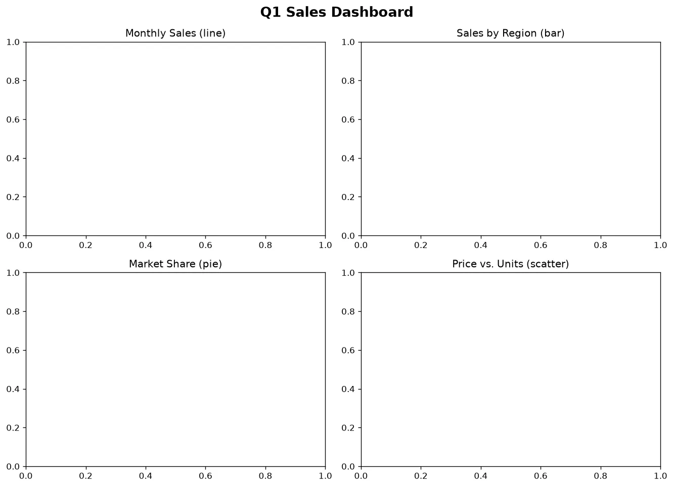
What you'll see: a single window split into four empty boxes arranged 2-by-2. Each box has its own title, and a bold super-title sits across the very top. This is the skeleton we'll now fill in.
2 Filling Every Panel
Now we draw a different chart type into each Axes using the object-oriented interface — ax.plot, ax.bar, ax.pie, and ax.scatter. Each panel keeps its own labels.
import matplotlib.pyplot as plt

months = ["Jan", "Feb", "Mar", "Apr", "May", "Jun"]
sales = [120, 135, 128, 160, 175, 190]
regions = ["North", "South", "East", "West"]
region_sales = [320, 280, 410, 360]
shares = [40, 25, 20, 15]
prices = [9.99, 12.5, 7.25, 15.0, 11.0, 8.5]
units = [200, 150, 320, 90, 170, 260]

fig, axs = plt.subplots(2, 2, figsize=(11, 8))

# Panel 1: line plot of monthly sales
axs[0, 0].plot(months, sales, marker="o", color="#3776AB")
axs[0, 0].set_title("Monthly Sales")
axs[0, 0].set_ylabel("Units sold")

# Panel 2: bar chart by region
axs[0, 1].bar(regions, region_sales, color="#2e8b57")
axs[0, 1].set_title("Sales by Region")

# Panel 3: pie chart of market share
axs[1, 0].pie(shares, labels=regions, autopct="%1.0f%%", startangle=90)
axs[1, 0].set_title("Market Share")

# Panel 4: scatter of price vs units
axs[1, 1].scatter(prices, units, c="#d2691e", s=80, alpha=0.7)
axs[1, 1].set_title("Price vs. Units")
axs[1, 1].set_xlabel("Price")
axs[1, 1].set_ylabel("Units")

fig.suptitle("Q1 Sales Dashboard", fontsize=16, fontweight="bold")
fig.tight_layout()
plt.show()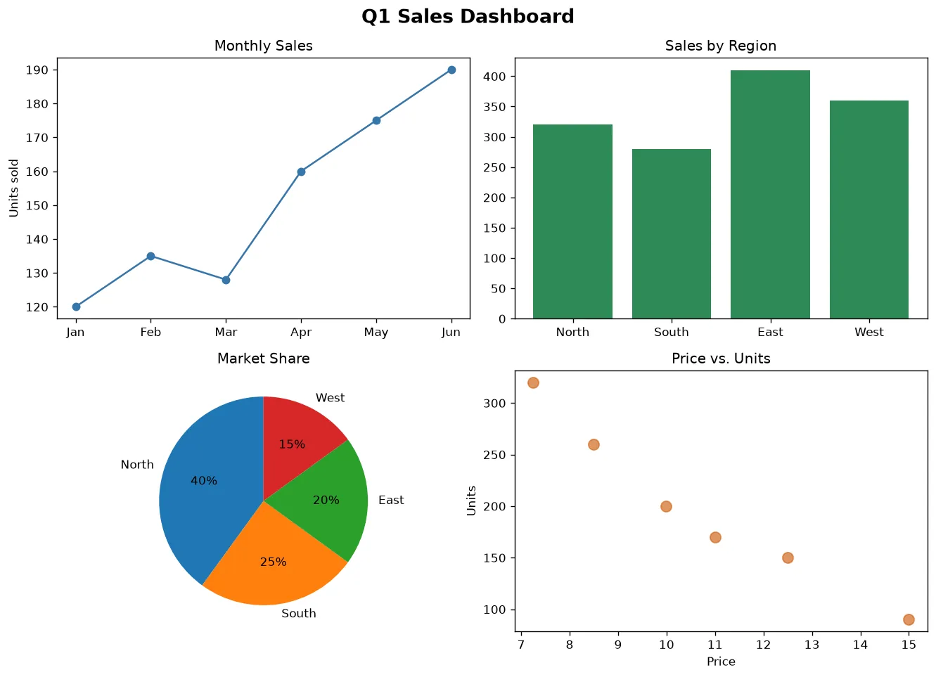
What you'll see: a polished four-panel dashboard. Top-left, a blue line with circle markers climbs across the six months. Top-right, four green bars compare regions. Bottom-left, a pie split into four labelled wedges with percentages. Bottom-right, orange dots scatter price against units. The bold title ties it all together.
3 Styling and Exporting
Finish by applying a consistent style with plt.style.use and saving the figure to disk with fig.savefig. Use bbox_inches="tight" to trim whitespace and a higher dpi for crisp output.
import matplotlib.pyplot as plt

# Apply a clean built-in theme to the whole figure
plt.style.use("seaborn-v0_8-whitegrid")

quarters = ["Q1", "Q2", "Q3", "Q4"]
revenue = [120, 150, 170, 210]
costs = [80, 95, 110, 130]

fig, (ax1, ax2) = plt.subplots(1, 2, figsize=(11, 4))

ax1.plot(quarters, revenue, marker="o", label="Revenue")
ax1.plot(quarters, costs, marker="s", label="Costs")
ax1.set_title("Revenue vs. Costs")
ax1.legend()

profit = [r - c for r, c in zip(revenue, costs)]
ax2.bar(quarters, profit, color="#2e8b57")
ax2.set_title("Profit by Quarter")

fig.suptitle("Annual Performance", fontsize=15, fontweight="bold")
fig.tight_layout()

# Export at high resolution BEFORE showing
fig.savefig("dashboard.png", dpi=150, bbox_inches="tight")
plt.show()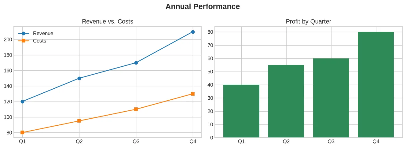
What you'll see: a clean two-panel figure on a soft white-grid theme. The left panel overlays revenue and cost lines with a legend; the right shows green profit bars. A file dashboard.png is written to your folder at 150 DPI with the margins trimmed tight.
🎯 Your Turn: Fill in the Blanks
Replace each ___ to finish this two-panel dashboard.
import matplotlib.pyplot as plt

days = ["Mon", "Tue", "Wed", "Thu", "Fri"]
visitors = [220, 260, 240, 300, 350]
signups = [12, 18, 15, 22, 30]

# Make a 1-row, 2-column grid of panels
fig, axs = plt.___(1, 2, figsize=(10, 4))

# Left panel: line plot of visitors
axs[0].___(days, visitors, marker="o")
axs[0].set_title("Daily Visitors")

# Right panel: bar chart of signups
axs[1].___(days, signups, color="teal")
axs[1].set_title("Daily Signups")

# One title for the whole figure
fig.___("Weekly Traffic Dashboard")

fig.tight_layout()
plt.show()
📋 Common Errors & Quick Reference
❌ Panels overlap each other
You forgot fig.tight_layout(). Call it after all panels are drawn, or pass constrained_layout=True to plt.subplots().
❌ TypeError: 'AxesSubplot' object is not subscriptable
With a single row or column, axs is 1D — index it as axs[0], not axs[0, 0]. The 2D form only works for a true grid like subplots(2, 2).
❌ Saved image is blank
Call fig.savefig(...) before plt.show() — showing the window clears the figure.
| Call | What It Does |
|---|---|
| plt.subplots(2, 2) | Make a grid of panels |
| axs[r, c].plot(...) | Draw into one panel |
| fig.suptitle(...) | One title for the figure |
| fig.tight_layout() | Auto-space the panels |
| fig.savefig("d.png", dpi=150) | Export the dashboard |
🏆 Mini Challenge: Your Own Three-Panel Dashboard
Build a 1×3 dashboard with a line, a bar, and a pie panel, then export it.
import matplotlib.pyplot as plt

plt.style.use("ggplot")

labels = ["A", "B", "C", "D"]
trend = [5, 9, 7, 12]
counts = [40, 25, 20, 15]

fig, axs = plt.subplots(1, 3, figsize=(13, 4))

# Panel 1 — line
axs[0].plot(labels, trend, marker="o")
axs[0].set_title("Trend")

# Panel 2 — bar
axs[1].bar(labels, counts, color="#3776AB")
axs[1].set_title("Counts")

# Panel 3 — pie
axs[2].pie(counts, labels=labels, autopct="%1.0f%%")
axs[2].set_title("Share")

fig.suptitle("My Capstone Dashboard", fontsize=15, fontweight="bold")
fig.tight_layout()
fig.savefig("my_dashboard.png", dpi=150, bbox_inches="tight")
plt.show()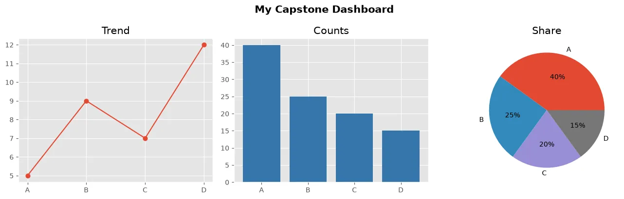
import matplotlib.pyplot as plt

months = ["Jan", "Feb", "Mar", "Apr"]
revenue = [120, 145, 132, 178]
costs = [90, 100, 95, 110]

fig, (top, bottom) = plt.subplots(2, 1, figsize=(7, 6), sharex=True)

top.plot(months, revenue, marker="o", label="revenue")
top.plot(months, costs, marker="s", label="costs")
top.set_ylabel("£000s")
top.legend()
top.set_title("A dashboard in two panels")

profit = [r - c for r, c in zip(revenue, costs)]
bars = bottom.bar(months, profit, color=["seagreen" if p > 35 else "grey" for p in profit])
bottom.set_ylabel("profit")

print("Panels:", len(fig.axes))
print("Lines on the top panel:", len(top.lines))
print("Profit per month:", profit)
print("Best month:", months[profit.index(max(profit))])
print("Bars highlighted green:", sum(1 for p in profit if p > 35))
print("Shared x axis:", top.get_shared_x_axes().joined(top, bottom))

# ✅ Expected output:
# Panels: 2
# Lines on the top panel: 2
# Profit per month: [30, 45, 37, 68]
# Best month: Apr
# Bars highlighted green: 3
# Shared x axis: True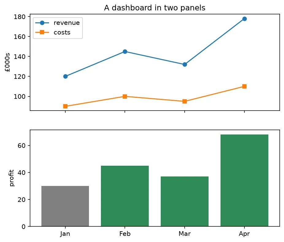
❓ Frequently Asked Questions
Course complete — you can now build full data dashboards!
From your first three-line chart to a styled, exported, multi-panel dashboard, you've covered the entire Matplotlib workflow: figures and axes, every core chart type, styling, annotations, dates, pandas integration, heatmaps, 3D, and global customization.
🚀 Keep going: rebuild one of these dashboards with your own real data — a budget, a fitness log, or a project's metrics. That's how the skills truly stick.
Practice quiz
What does plt.subplots(2, 2) return?
- The figure plus a 2D array of Axes
- Only a figure
- A single Axes
- A list of figures
Answer: The figure plus a 2D array of Axes. It returns (fig, axs) where axs is a 2x2 array of Axes you index as axs[row, col].
How do you index the top-right panel of a 2x2 grid?
- axs[1]
- axs[0, 1]
- axs[2]
- axs.right
Answer: axs[0, 1]. In a true 2D grid you index axs[row, col]; top-right is axs[0, 1].
Which call gives the whole figure one super-title?
- ax.set_title()
- plt.xlabel()
- fig.suptitle('...')
- fig.title()
Answer: fig.suptitle('...'). fig.suptitle() places a single title above all panels.
Which call stops subplots from overlapping?
- fig.clear()
- plt.legend()
- fig.show()
- fig.tight_layout()
Answer: fig.tight_layout(). fig.tight_layout() auto-adjusts spacing so labels and titles don't collide.
Why use the object-oriented interface (ax.plot) for a multi-panel dashboard?
- It removes ambiguity about which panel you mean
- It is faster to type
- It enables animation
- It is the only way to set colors
Answer: It removes ambiguity about which panel you mean. With several panels, plt.plot() can't tell which Axes you mean; ax methods are explicit.
When should you call fig.savefig() relative to plt.show()?
- After plt.show()
- Before plt.show()
- It does not matter
- Only inside a loop
Answer: Before plt.show(). Save before showing; showing the window can clear the figure, giving a blank image.
Which savefig argument trims surrounding whitespace?
- dpi=150
- transparent=True
- bbox_inches='tight'
- format='png'
Answer: bbox_inches='tight'. bbox_inches='tight' crops the saved image to its content.
With plt.subplots(1, 2), how is axs indexed?
- axs[0, 0]
- axs['left']
- axs.first
- axs[0] and axs[1] (it is 1D)
Answer: axs[0] and axs[1] (it is 1D). A single row gives a 1D array, so use axs[0], not axs[0, 0].
Which method draws a pie chart into a specific panel?
- axs[1, 0].pie(...)
- plt.pie() globally
- fig.pie(...)
- axs.pie_all()
Answer: axs[1, 0].pie(...). Call .pie() on the specific Axes, e.g. axs[1, 0].pie(...).
What controls the resolution of a saved figure?
- bbox_inches
- dpi
- figsize only
- startangle
Answer: dpi. dpi (dots per inch) sets the output resolution, e.g. dpi=150.
Continue this course
- Previous: Checkpoint: Data Visualization
- Quick reference: Matplotlib cheat sheet
Frequently asked questions
What is a dashboard in Matplotlib?
A dashboard is a single figure that combines several related charts — line, bar, pie, scatter — into one coordinated view, usually built with plt.subplots() so every panel shares the same figure.
How do I stop subplots from overlapping?
Call fig.tight_layout() (or plt.tight_layout()) after adding all your plots. It automatically adjusts spacing so titles, labels, and ticks don't collide. constrained_layout=True in plt.subplots() does the same job proactively.
Can I give the whole dashboard one title?
Yes. Use fig.suptitle('My Dashboard') for a single super-title above all panels, separate from each subplot's own ax.set_title().
How do I export a finished dashboard?
Call fig.savefig('dashboard.png', dpi=150, bbox_inches='tight') before plt.show(). bbox_inches='tight' trims surrounding whitespace and dpi controls the resolution.