Text, Math & LaTeX in Plots
Reviewed & published by Brayan K
Annotations are the words, arrows, and equations you layer onto a chart to point out features and explain what the reader is looking at.
Part of the free Matplotlib course at LearnCodingFast — hands-on lessons with worked examples and the output they print, plus practice exercises and a quick quiz.
In this lesson you'll place text with ax.text(), draw labeled arrows with ax.annotate(), pin labels to corners with transAxes, and typeset equations using mathtext between dollar signs.
What You'll Learn in This Lesson
- Placing text with ax.text() at data points
- Drawing labeled arrows with ax.annotate()
- Positioning xy versus xytext
- Pinning labels to corners with transAxes
- Typesetting math between dollar signs
- Styling with fontsize, weight, and bbox
1 Placing Text with ax.text()
The simplest annotation is ax.text(x, y, "label"), which drops a string at the data coordinate you give. Style it with fontsize, color, and weight. Because the position is in data units, the text follows your data if the axes rescale.
import matplotlib.pyplot as plt
import numpy as np

x = np.linspace(0, 10, 100)
y = np.sin(x)

fig, ax = plt.subplots(figsize=(7, 4), constrained_layout=True)
ax.plot(x, y)

# Place plain text at a data coordinate
ax.text(5, 0.8, "Here is some text",
        fontsize=12, color="darkred", weight="bold")

ax.set_title("Adding Text at Data Coordinates")
plt.show()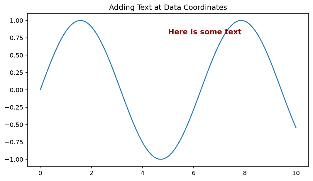
What you'll see: a sine wave with the bold, dark-red phrase "Here is some text" floating near the top of the plot at x = 5, y = 0.8.
2 Labeled Arrows with ax.annotate()
To point at a feature, use ax.annotate(). Give it the target point with xy, the label position with xytext, and an arrowprops dictionary to draw the connector. This is the standard way to call out a peak, an outlier, or a region of interest.
import matplotlib.pyplot as plt
import numpy as np

x = np.linspace(0, 10, 200)
y = np.sin(x)

fig, ax = plt.subplots(figsize=(7, 4), constrained_layout=True)
ax.plot(x, y)

# Find the highest point and annotate it with an arrow
peak_x = x[np.argmax(y)]
peak_y = y.max()

ax.annotate("Peak!",
            xy=(peak_x, peak_y),                  # the point to mark
            xytext=(peak_x + 1.5, peak_y + 0.4),  # where the label sits
            arrowprops=dict(arrowstyle="->", color="black"),
            fontsize=12)

ax.set_title("Annotating a Peak")
plt.show()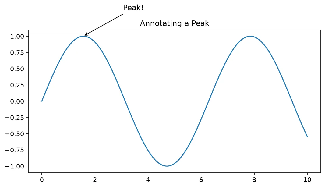
What you'll see: a sine wave with the word "Peak!" sitting just above and to the right of the first crest, connected to the exact peak point by a thin arrow.
3 Math with $...$ and transAxes
Wrap an expression in dollar signs to render it as math, and use a raw string (the r"..." prefix) so backslash commands like \sqrt survive. To pin a label to a corner regardless of the data, pass transform=ax.transAxes, which switches to axes-fraction coordinates from (0, 0) at the bottom-left to (1, 1) at the top-right.
import matplotlib.pyplot as plt
import numpy as np

x = np.linspace(-3, 3, 200)
y = np.exp(-x**2)

fig, ax = plt.subplots(figsize=(7, 4), constrained_layout=True)
ax.plot(x, y, color="purple")

# Mathtext uses $...$ in a RAW string so backslashes survive
ax.set_title(r"Gaussian: $f(x) = e^{-x^2}$", fontsize=14)
ax.set_xlabel(r"$x$")
ax.set_ylabel(r"$f(x)$")

# Place a boxed formula using axes-fraction coordinates (0..1)
ax.text(0.05, 0.9, r"$\int_{-\infty}^{\infty} e^{-x^2}\,dx = \sqrt{\pi}$",
        transform=ax.transAxes, fontsize=12,
        bbox=dict(boxstyle="round", facecolor="wheat", alpha=0.7))

plt.show()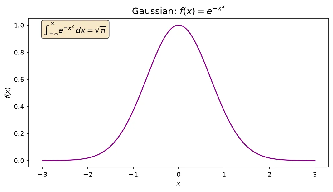
What you'll see: a purple bell curve titled with the rendered equation f(x) = e to the minus x squared, axis labels in italic math, and a rounded wheat-colored box in the top-left holding the Gaussian integral that equals the square root of pi.
🎯 Your Turn: Fill in the Blanks
Replace each ___ to pin a label to the top-left corner using axes coordinates.
import matplotlib.pyplot as plt
import numpy as np

x = np.linspace(0, 6, 100)
y = x**2

fig, ax = plt.subplots(figsize=(7, 4), constrained_layout=True)
ax.plot(x, y)

# Place a label at axes-fraction (0.05, 0.9) -> the top-left corner.
# Switch to axes coordinates so the position ignores the data.
ax.text(0.05, 0.9, "Quadratic growth",
        transform=ax.___, fontsize=12, weight="bold")

ax.set_title("y = x squared")
plt.show()
Hint: the axes-fraction transform is ax.transAxes.
📋 Common Errors & Quick Reference
❌ My equation shows raw backslashes
You forgot the raw-string prefix. Use r"$\sqrt{x}$" so Python doesn't eat the backslash before Matplotlib renders it.
❌ My text moves when the data changes
You placed it in data coordinates. Add transform=ax.transAxes to pin it to a fixed spot on the Axes instead.
❌ No arrow appears with annotate()
An arrow only shows when you pass arrowprops. Without it, annotate behaves like plain text.
| Call | What It Does |
|---|---|
| ax.text(x, y, s) | Plain label at a point |
| ax.annotate(s, xy=, xytext=) | Label with an arrow |
| transform=ax.transAxes | Use axes-fraction coordinates |
| r"$...$" | Render math via mathtext |
🏆 Mini Challenge: Annotated Decay Curve
Plot a damped oscillation with a mathtext title, an arrow pointing at the first trough, and a boxed mathtext note pinned to a corner.
import matplotlib.pyplot as plt
import numpy as np

t = np.linspace(0, 5, 200)
y = np.exp(-t) * np.cos(2 * np.pi * t)

fig, ax = plt.subplots(figsize=(8, 4), constrained_layout=True)
ax.plot(t, y, color="teal")

# Mathtext title using a raw string
ax.set_title(r"Damped Oscillation: $e^{-t}\cos(2\pi t)$", fontsize=14)

# Arrow annotation pointing at the first trough
ax.annotate("first trough",
            xy=(0.5, np.exp(-0.5) * np.cos(np.pi)),
            xytext=(2, -0.6),
            arrowprops=dict(arrowstyle="->", color="crimson"),
            fontsize=11)

# A boxed note pinned to the axes corner
ax.text(0.97, 0.95, r"amplitude $\propto e^{-t}$",
        transform=ax.transAxes, ha="right", va="top",
        bbox=dict(boxstyle="round", facecolor="lightyellow"))

plt.show()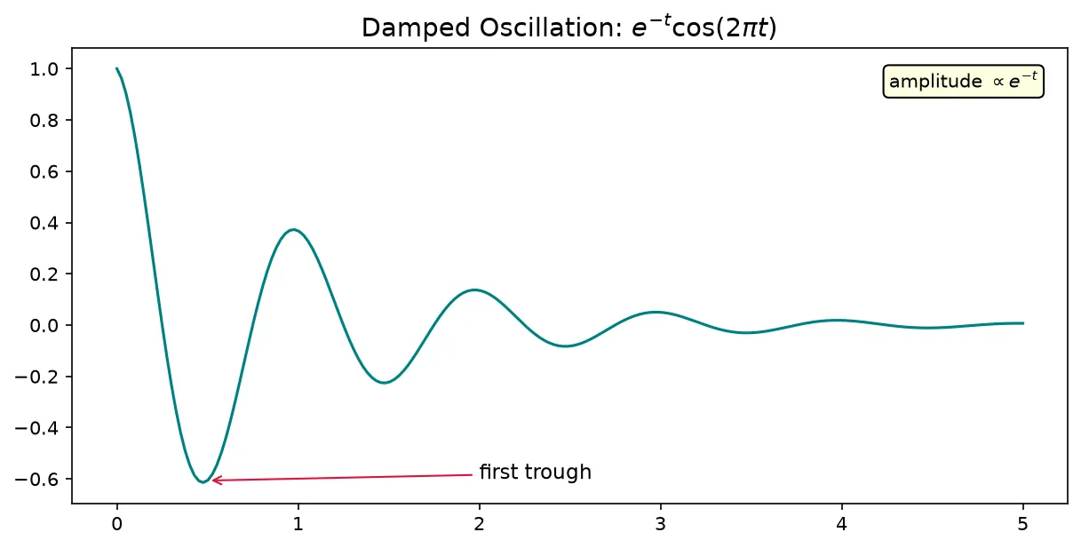
import matplotlib.pyplot as plt

fig, ax = plt.subplots()
ax.set_xlim(0, 4)
ax.set_ylim(0, 4)

plain = ax.text(0.5, 3.0, "plain text")
maths = ax.text(0.5, 2.0, r"$E = mc^2$")
sub = ax.text(0.5, 1.0, r"$H_2O$ and $x^{n+1}$")
ax.set_title(r"Speed: $v = \frac{d}{t}$")

print("Text objects:", len(ax.texts))
print("Plain:", plain.get_text())
print("Maths source stays as you typed it:", maths.get_text())
print("Subscript and superscript:", sub.get_text())
print("Title:", ax.get_title())
print("Dollar signs mark the maths:", maths.get_text().startswith("$") and maths.get_text().endswith("$"))

# ✅ Expected output:
# Text objects: 3
# Plain: plain text
# Maths source stays as you typed it: $E = mc^2$
# Subscript and superscript: $H_2O$ and $x^{n+1}$
# Title: Speed: $v = \frac{d}{t}$
# Dollar signs mark the maths: True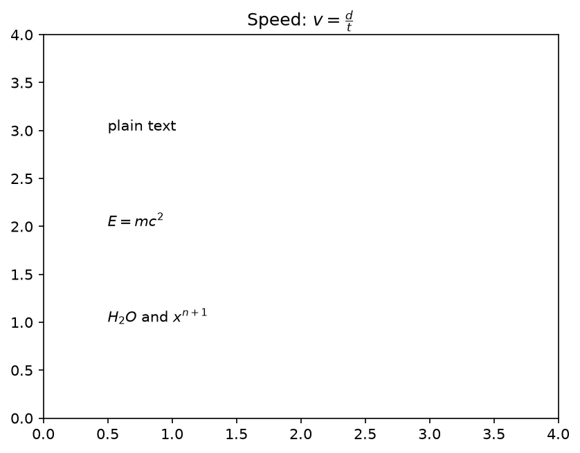
❓ Frequently Asked Questions
Lesson complete — your charts can speak for themselves!
You placed text with ax.text(), drew labeled arrows with ax.annotate(), pinned labels using transAxes, and typeset equations with mathtext between dollar signs.
Practice quiz
Which call drops a plain string at a data coordinate?
- ax.label(x, y, 'hi')
- ax.put(x, y, 'hi')
- ax.text(x, y, 'hi')
- ax.write(x, y, 'hi')
Answer: ax.text(x, y, 'hi'). ax.text(x, y, 'label') places a plain string at the given data coordinate.
What is ax.annotate() specifically built for?
- Saving figures
- Resizing axes
- Setting the colormap
- Callouts with an arrow pointing at a feature
Answer: Callouts with an arrow pointing at a feature. annotate() takes xy, xytext, and arrowprops to draw a labeled arrow.
In ax.annotate(), which argument is the point being marked?
- xy
- xytext
- point
- target
Answer: xy. xy is the point to mark; xytext is where the label text sits.
What makes annotate() draw an arrow rather than plain text?
- color=
- arrowprops=
- marker=
- linestyle=
Answer: arrowprops=. An arrow only appears when you pass an arrowprops dictionary.
How do you switch into Matplotlib's math rendering (mathtext)?
- Wrap text in #...#
- Use math=True
- Wrap the expression in dollar signs $...$
- Use ax.math()
Answer: Wrap the expression in dollar signs $...$. Mathtext is enabled by wrapping the expression in dollar signs, e.g. $E=mc^2$.
Why use a raw string r'...' for a mathtext label?
- It centers the text
- It makes the font bold
- It enables LaTeX install
- So backslash commands like \sqrt are passed through literally
Answer: So backslash commands like \sqrt are passed through literally. A raw string keeps backslashes intact so commands like \alpha survive.
What does transform=ax.transAxes switch the coordinates to?
- Axes-fraction coordinates from (0,0) to (1,1)
- Pixel coordinates
- Polar coordinates
- Inches from the origin
Answer: Axes-fraction coordinates from (0,0) to (1,1). transAxes uses axes-fraction coordinates, with (0,0) bottom-left and (1,1) top-right.
Which dictionary draws a box around text?
- box=dict(...)
- bbox=dict(boxstyle='round', facecolor='wheat')
- frame=dict(...)
- border=dict(...)
Answer: bbox=dict(boxstyle='round', facecolor='wheat'). Pass a bbox dictionary with boxstyle, facecolor, and alpha to box the text.
In mathtext, how do you write a superscript like x squared?
- x*2
- x#2
- x^2
- x~2
Answer: x^2. Superscripts use ^ and subscripts use _ in mathtext, with braces to group.
Is a LaTeX installation required to use mathtext?
- No — mathtext works out of the box
- Yes, always
- Only on Windows
- Only for subscripts
Answer: No — mathtext works out of the box. Mathtext is built in and needs no external LaTeX install.
Continue this course
- Previous: Tick Locators & Formatters
- Next: Animations (FuncAnimation) — Build frame-by-frame animations and export them to GIF/MP4
- Quick reference: Matplotlib cheat sheet
Frequently asked questions
What is the difference between ax.text() and ax.annotate()?
ax.text(x, y, 'label') simply drops a string at a point. ax.annotate() is built for callouts: it takes the point to mark with xy, the place to put the label with xytext, and an arrowprops dictionary so an arrow connects the two. Use text for a plain note and annotate when you want an arrow pointing at something.
How do I write math or equations in a Matplotlib label?
Wrap the math in dollar signs to switch into mathtext, Matplotlib's built-in TeX-like renderer: ax.set_title(r'$E = mc^2$'). Use a raw string (the r prefix) so backslashes in commands like \alpha or \sqrt are passed through literally instead of being treated as escape characters.
What does transform=ax.transAxes do?
By default text coordinates are in data units. transform=ax.transAxes switches to axes-fraction coordinates where (0, 0) is the bottom-left corner and (1, 1) is the top-right, regardless of the data. It is the reliable way to pin a label to a corner of the plot no matter how the data scales.
How do I put a box around my text?
Pass a bbox dictionary: bbox=dict(boxstyle='round', facecolor='wheat', alpha=0.7). boxstyle controls the shape (round, square), facecolor the fill, and alpha the transparency. The same bbox argument works on both ax.text() and ax.annotate().